Flow around three squares side by side

Table of Contents

1. Presentation of the test case
2. Configuration files
- 2.1. cfg file
- 2.2. json file
Bibliography

1. Presentation of the test case

1.1. Presentation

This study is based on the flow of a fluid in front of three side-by-side square cylinders. The cylinders are arranged side by side, the center of the central cylinder represents the origin of the coordinate system, one of the two other cylinders is placed below the central cylinder and the other above.

In this test case, we are particularly interested in the effect of the spacing ratio L/W on the flow, where L is the center-to-center spacing of the cylinder and W is the cylinder side width.

The numerical results obtained in this study will be compared with those found in the literature, for different gaps \(L/W < 1.4\) and \(L/W \in [1.4,9\)] with a Reynolds number equal to \(Re=150\).

1.2. Geometry setting

The arrangement of the cylinders in the calculation area \(\Omega\) is shown in the figure below :

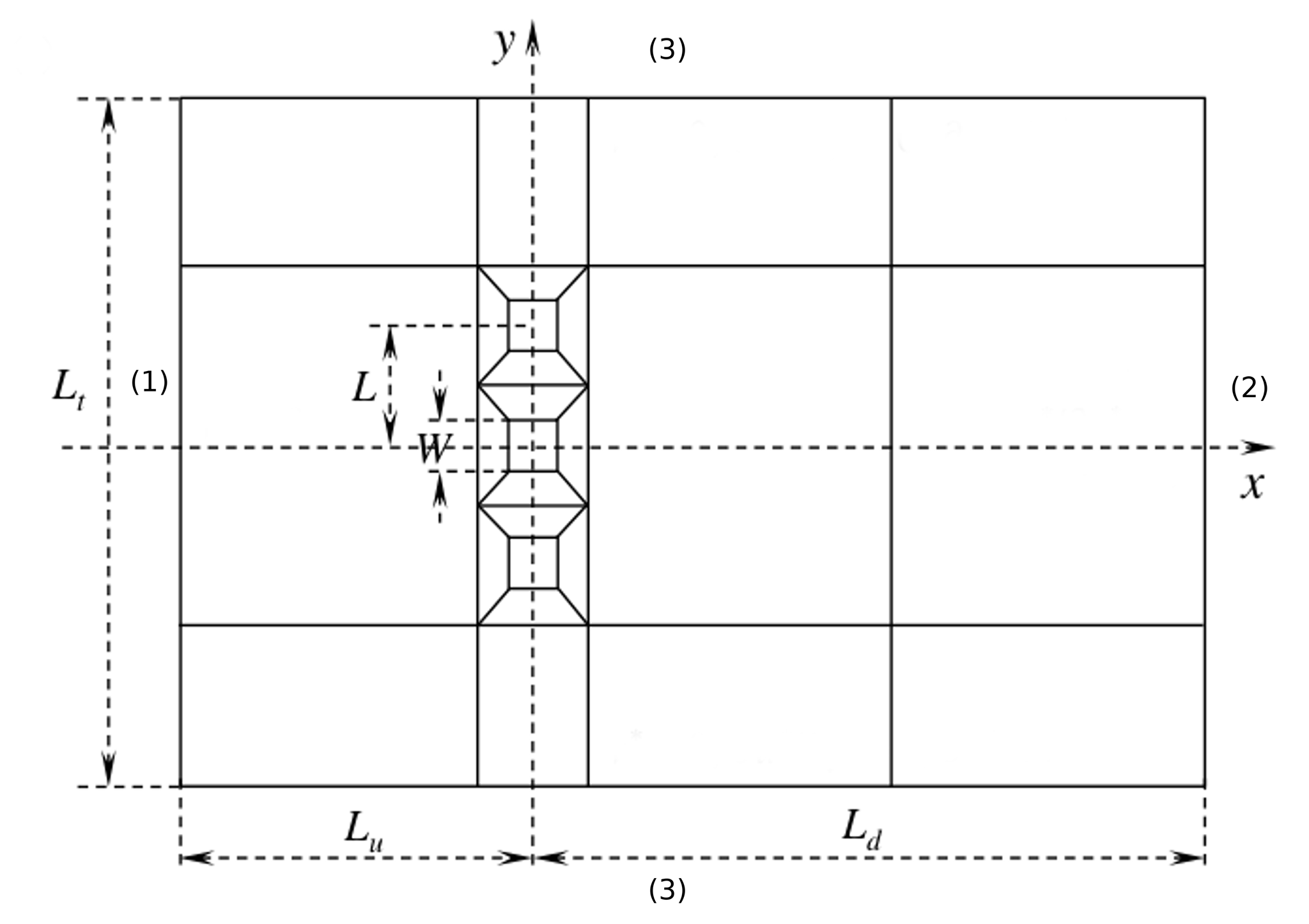
Figure 1. The geometric setting for the 3 cylinder with central cylinder represents the origin of the coordinate system

We provide here the basic geometry used in Gmsh to describe \(\Omega\).

Geo file

// Gmsh project created on Sat Aug  8 13:20:47 2020
w=2;
l_sur_w=1.5;
l=w*(l_sur_w);
Lt=w/(5.26/100);
Ld=29.5*w;
Lu=13.5*w;
h=0.5;
//+grand caree (domaine)
Point(1) = {0, 0, 0, h};
//+
Point(2) = {Ld, Lt/2, 0, h};
//+
Point(3) = {Ld, -Lt/2, 0, h};
//+
Point(4) = {- Lu, Lt/2, 0, h};
//+
Point(5) = {- Lu, -Lt/2, 0, h};
//+
Line(1) = {4, 5};
//+
Line(2) = {5, 3};
//+
Line(3) = {3, 2};
//+
Line(4) = {2, 4};
//+zone des caree
//Point(6) = {5, Lt/2, 0, 1.0};
//+
//Point(7) = {-5, Lt/2, 0, 1.0};
//+
//Point(8) = {5, -Lt/2, 0, 1.0};
//+
//Point(9) = {-5, -Lt/2, 0, 1.0};
//+
//Line(5) = {7, 9};
//+
//Line(6) = {6, 8};
//caree milieu
Point(10) = {w/2,w/2, 0, h};
Point(11) = {-w/2,w/2, 0, h};
Point(12) = {w/2,-w/2, 0, h};
Point(13) = {-w/2,-w/2, 0, h};
Line(7) = {10, 11};
Line(8) = {11, 13};
Line(9) = {13, 12};
Line(10) = {12, 10};
//caree haut
Point(14) = {0,l, 0, h};
Point(15) = {w/2,l+w/2, 0, h};
Point(16) = {-w/2,l+w/2, 0, h};
Point(17) = {w/2,l-w/2, 0, h};
Point(18) = {-w/2,l-w/2, 0, h};
Line(11) = {17, 18};
Line(12) = {18, 16};
Line(13) = {16, 15};
Line(14) = {15, 17};
//caree bas
Point(19) = {0,-l, 0, h};
Point(20) = {w/2,-l+w/2, 0, h};
Point(21) = {-w/2,-l+w/2, 0, h};
Point(22) = {w/2,-l-w/2, 0, h};
Point(23) = {-w/2,-l-w/2, 0, h};

//+
Line(15) = {20, 21};
//+
Line(16) = {21, 23};
//+
Line(17) = {23, 22};
//+
Line(18) = {22, 20};
//+
Line Loop(1) = {4, 1, 2, 3};
//+
Line Loop(2) = {13, 14, 11, 12};
//+
Line Loop(3) = {7, 8, 9, 10};
//+
Line Loop(4) = {15, 16, 17, 18};
//+
Plane Surface(1) = {1, 2, 3, 4};
//+
Physical Line("inlet") = {1};
//+
Physical Line("outlet") = {3};
//+
Physical Line("wall1") = {4};
//+
Physical Line("wall2") = {2};
//+
Physical Surface("omega") = {1};

The Data provided on the whole \(\Omega\) domain allows us to have conditions at the specified limits, the table below summarize these data.

Table 1. Geometric data table
Notation	Description	Value	Unit
\(W\)	cylinder width	-	\(m\)
\(L\)	the center-to-center spacing of the cylinder	-	\(m\)
\(L_t\)	side of the domain	\(W\frac{1}{5.26\%}\)	\(m\)
\(L_u\)	upstream boundary separations from the coordinate origin	\(13.5W\)	\(m\)
\(L_d\)	downstream boundary separations from the coordinate origin	\(29.5W\)	\(m\)
\(U\)	Inlet velocity	1	\(m/s\)

1.3. Physical setting

The Physical parameters are:

Table 2. Physical data table
Notation	Description	Value	Unit
\(\rho\)	Density	1	\(Kg/m^3\)
\(\mu\)	Dynamic viscosity	1	\(Pa.s\)

1.4. Boundary conditions

In this study 3 boundary conditions are imposed: Inlet condition, Outlet condition and the Wall condition.

Inlet condition

On boundary (1) a Dirichlet-type condition is imposed and a Poiseuille profile is placed as an entry condition, it’s defined by:

\[u = U \\ v = 0\]

json configuration for the inlet boundary condition

"Dirichlet":
{
    "inlet":
    {
       "expr":"{1,0}"
    }
 },

Wall conditions

On the limits (3), i.e. on the upper and lower wall we have :

\[\frac{\partial{u}}{\partial{y}}=0\\ \frac{\partial{p}}{\partial{y}}=0\\ v=0\]

json configuration for the wall boundary condition

"outlet":
{
     "wall1":
     {
         "expr":"0"
     },
     "wall2":
     {
         "expr":"0"
     }
}

Outlet condition

On boundary (2) (i.e the exit boundary condition) a Neumann-type condition is imposed

\[\frac{\partial{u}}{\partial{x}}=0\\ \frac{\partial{v}}{\partial{x}}=0\\ \frac{\partial{p}}{\partial{x}}=0\]

json configuration for the outlet boundary condition

"Neumann_scalar":
 {
     "outlet":
      {
          "expr":"0"
      }
 }

1.5. Mesh

We move on to meshing to generate fully structured uniform triangular cells, the figure below shows a part of the generated mesh:

Figure 2. generated mesh for case \(L/W = 1.5\)

Figure 3. represents a zoom-in view of the previous mesh

2. Configuration files

2.1. cfg file

directory=resulats/caree/P1

[case]
discretization= P2P1G1
dimension=2

[fluid]
filename=$cfgdir/caree.json
mesh.filename=$cfgdir/caree.geo
gmsh.hsize=0.5

solver= Newton #Oseen #Newton #Picard,Newton
linearsystem-cst-update=false
jacobian-linear-update=false

snes-monitor=true
pc-type= gams #gasm,lu

[fluid.bdf]
order=2

[ts]
time-step=0.1
time-final=5

2.2. json file

Here the full json configuration file

Json file

{
    "Name": "three squares side by side",
    "ShortName":"flow past",
    "Models":
    {
         "equations": "Navier-Stokes"
    },
    "Materials":
    {
        "omega":
        {
            "rho":"1",
            "mu":"1"
        }
    },
    "BoundaryConditions":
    {
        "velocity":
        {
            // tag::inlet[]
            "Dirichlet":
            {
                "inlet":
                {
                   "expr":"{1,0}"
                }
             },
            // end::inlet[]

            // tag::walls[]
            "outlet":
            {
                 "wall1":
                 {
                     "expr":"0"
                 },
                 "wall2":
                 {
                     "expr":"0"
                 }
            }
           // end::walls[]
        },
        "fluid":
        {
          // tag::outlet[]
          "Neumann_scalar":
           {
               "outlet":
                {
                    "expr":"0"
                }
           }
          // end::outlet[]
        }
    },
    "PostProcess":
    {
        "Exports":
        {
            "fields":["velocity","pressure"]
        }
    }
}

Bibliography

[zheng-2019] Forces and flow around three side-by-side square cylinders, Qinmin Zheng, Md. Mahbub Alam, October 2019 Wind and Structures An International Journal 29(1):1-13 DOI: 10.12989/was.2019.29.1.001 Download PDF