Laminar isothermal backward facing step
1. Presentation of the test case
1.1. Presentation
This study will be based on a laminar flow around a step laid in a flat channel. The fluid is subjected to a sudden widening that causes an inverse pressure gradient, where the flow separates into several zones, among which is formed a recirculation zone noted \(x_r\) where the flow closes to return to the step.
The Reynolds number denoted Re for this flow is calculated from the channel height S, the average flow velocity \(U_{ave}\) and the kinematic viscosity v, and is defined by:
And as \(v=\frac{\mu}{\rho}\) so:
When the flow has low Reynolds number values, it is said to be stationary, while flows with higher
Reynolds number values become turbulent and the average length of the recirculation zone decreases
until a constant saturation value is reached. In this case, we are only interested in two different
Reynolds number values: Re=389 and Re=1095.
1.2. Geometry setting
The computational domain \(\Omega\) is a channel with a descending step as shown in the figure below :
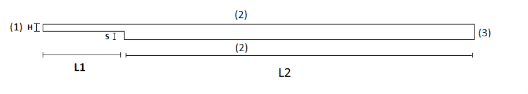
We provide here the basic geometry used in Gmsh to describe \(\Omega\).
// Gmsh project created on Mon Apr 27 18:52:15 2020
//+
h=5e-4;
S=0.0049;
H=0.0052;
L1=0.2;
L2=0.5;
//Points
Point(3) = {0, 0, 0, h};
Point(4) = {L2, 0, 0, h};
Point(5) = {-L1, S, 0, h};//+0.0049
Point(6) = {0, S, 0, h};
Point(7) = {-L1, S+H, 0, h};//+0.0101
Point(8) = {L2, S+H, 0, h};
//Line basique
Line(1) = {7, 5};
Line(2) = {5, 6};
Line(3) = {6, 3};
Line(4) = {3, 4};
Line(5) = {4, 8};
Line(6) = {8, 7};
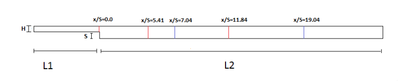
//Points vertical 1er cas re=398
Point(9) = {0, S+H, 0, h};
Point(10) = {S*5.41, 0, 0, h};
Point(11) = {S*5.41, S+H, 0, h};
Point(12) = {S*11.84, 0, 0, h};
Point(13) = {S*11.84, S+H, 0, h};
//Points vertical 2eme cas re=1095
Point(14) = {S*7.04, 0, 0, h};
Point(15) = {S*7.04, S+H, 0, h};
Point(16) = {S*19.04, 0, 0, h};
Point(17) = {S*19.04, S+H, 0, h};
//+marker pour Re=389
Line(7) = {9, 6};
Line(8) = {11, 10};
Line(9) = {13, 12};
Physical Line("marker_L1") = {7};
Physical Line("marker_L2") = {8};
Physical Line("marker_L3") = {9};
//marker pour Re=1095
Line(25) = {15, 14};
Line(26) = {17, 16};
Physical Line("marker_L4") = {25};
Physical Line("marker_L5") = {26};
Physical Point("pt1")={7};
Physical Point("pt2")={9};
Physical Point("pt3")={11};
Physical Point("pt4")={15};
Physical Point("pt5")={13};
Physical Point("pt6")={17};
Physical Point("pt7")={8};
//+
Line Loop(1) = {6, 1, 2, 3, 4, 5};
Plane Surface(1) = {1};
Delete {
Surface{1};
}
Delete {
Line{2}; Line{1}; Line{6}; Line{4}; Line{3}; Line{5};
}
//entee
Line(10) = {7, 5};
//sortie
Line(11) = {4, 8};
//sortie---->entree
Line(12) = {8, 17};
Line(13) = {17, 13};
Line(14) = {13, 15};
Line(15) = {15, 11};
Line(16) = {11, 9};
Line(17) = {9, 7};
//entree--->sortie
Line(18) = {5, 6};
Line(19) = {6, 3};
Line(20) = {3, 10};
Line(21) = {10, 14};
Line(22) = {14, 12};
Line(23) = {12, 16};
Line(24) = {16, 4};
//surface
Line Loop(2) = {12, 26, 24, 11};
Plane Surface(1) = {2};
Line Loop(3) = {13, 9, 23, -26};
Plane Surface(2) = {3};
Line Loop(4) = {14, 25, 22,-9};
Plane Surface(3) = {4};
Line Loop(5) = {15, 8, 21,-25};
Plane Surface(4) = {5};
Line Loop(6) = {16, 7, 19, 20, -8};
Plane Surface(5) = {6};
Line Loop(7) = {17, 10, 18, -7};
Plane Surface(6) = {7};
//phy surface
Physical Surface("omega") = {1, 2, 3, 4, 5, 6};
//phy line
Physical Line("inlet") = {10};
Physical Line("outlet") = {11};
Physical Line("wall1") = {20,21,22,23,24};
Physical Line("wall2") = {19,18};
Physical Line("wall3") = {17,16,15,14,13,12};The Data provided on the whole \(\Omega\) domain allows us to have conditions at the specified limits, the table below summarize these data.
| Notation | Description | Value | Unit |
|---|---|---|---|
\(L1\) |
Length of the upstream section |
2e-1 |
\(m\) |
\(L2\) |
Length of the downstream section |
5e-1 |
\(m\) |
\(S\) |
Step height |
4.9e-3 |
\(m\) |
\(H\) |
Inlet channel height |
5.2e-3 |
\(m\) |
\(U_{int}\) |
Inlet velocity |
- |
\(m/s\) |
\(U_{ave}\) |
Average velocity |
- |
\(m\)/s |
1.3. Physical setting
The Physical parameters are:
| Notation | Description | Value | Unit |
|---|---|---|---|
\(\rho\) |
Density |
1.23 |
\(Kg/m^3\) |
\(\mu\) |
Dynamic viscosity |
1.79e-5 |
\(Pa.s\) |
\(v\) |
Kinematic viscosity |
1.4553e-5 |
\(m^2/s\) |
1.4. Boundary conditions
In this study 3 boundary conditions are imposed:
-
Inlet condition
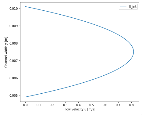
On boundary (1) a Poiseuille profile is placed as an entry condition, it is defined by:
such as \(y_1=y-S\), and \(U_{ave}\) are derived from the selected Reynolds number as:
"inlet":
{
    "expr":"{6*uave*((y-s)/h)*(1-((y-s)/h)),0}:uave:s:h:y"
},
At the entrance the profile of Poiseuille is represented by the graphe below:
-
For
Re=389:
-
For
Re=1095:
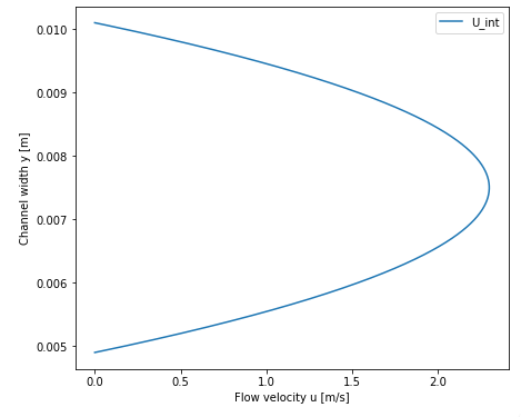
-
Wall conditions
On the limits (2), i.e. on the upper and lower wall we have :
"wall1":
{
    "expr":"{0,0}"
},
"wall2":
{
    "expr":"{0,0}"
},
"wall3":
{
    "expr":"{0,0}"
}-
Outlet condition
On boundary (3) the exit boundary condition is free, which means that no constraint is imposed on the exit boundary.
"outlet":
{
    "expr":"0"
}
1.5. Conformal blocks division
To study the laminar flow around a backward Facing Step we have devised the geometry in conformal blocks as the figure below illustrates:
1.6. Mesh
After cutting our domain, we move on to meshing to generate fully structured uniform triangular cells, the figure below shows a part of the generated mesh:
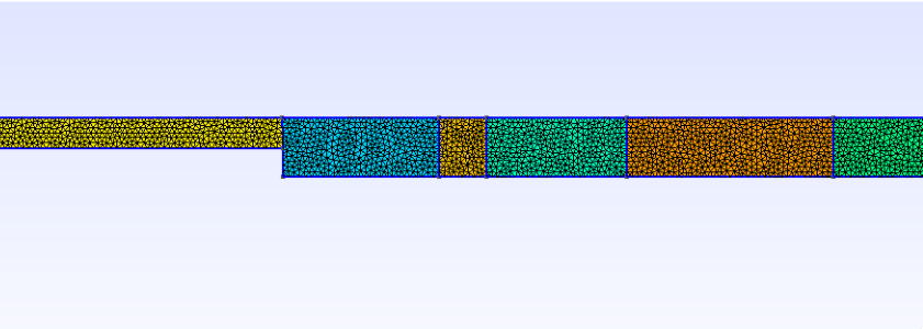
The study will be based on velocity profiles at different downstream locations, represented by
the different vertical lines \(x/S\) for Re = 389 and Re = 1095.
2. Results
For the readability of the results, we have separated the calculations for Re= 389 and those for
Re=1095.
|
2.1. Running the case:
The command line to run this cases is
mpirun -np 4 feelpp_toolbox_fluid--config-file laminar.cfg--fluid.snes-monitor=1--fluid.gmsh.hsize=3e-4Once the command is executed the results are exported to ParaView for viewing the flow by executing:
rsync -avz atlas.math.unistra.fr:/feel2.2. Results for Re=389
In this part the problem is dealt with in a stationary frame.
| The solution does not depend on the time, more precisely the flow profile is to long at the points where the flow variation is not visible. |
2.2.1. Configuration files
json file
{
    "Name": "Laminar, Isothermal Backward Facing Step Benchmark",
    "ShortName":"ecoulementinstationnaire",
    "Models":
    {
         "equations": "Navier-Stokes"
    },
    "Parameters":
    {
        "h":"5.2e-3",
        "s":"4.9e-3",
        "uave":"0.54433"
    },
    "Materials":
    {
        "omega":
        {
            "rho":"1.23",
            "mu":"1.79e-5"
        }
    },
    "BoundaryConditions":
    {
        "velocity":
        {
            "Dirichlet":
            {   // tag::inlet[]
                "inlet":
                {
                    "expr":"{6*uave*((y-s)/h)*(1-((y-s)/h)),0}:uave:s:h:y"
                },
               // end::inlet[]

               // tag::walls[]
                "wall1":
                {
                    "expr":"{0,0}"
                },
                "wall2":
                {
                    "expr":"{0,0}"
                },
                "wall3":
                {
                    "expr":"{0,0}"
                }
                // end::walls[]
            }
        },
        "fluid":
        {
            "outlet":
            {
               // tag::outlet[]
                "outlet":
                {
                    "expr":"0"
                }
              // end::outlet[]
            }
        }
    },
    "PostProcess":
    {
        "Exports":
        {
            "fields":["velocity"]
        }

    }
}
cfg file
directory=resulats/stationnaire389/P1
[case]
discretization= P2P1G1
dimension=2
[fluid]
filename=$cfgdir/laminar.json
mesh.filename=$cfgdir/laminar.geo
gmsh.hsize=0.0005
solver= Newton #Oseen #Newton #Picard,Newton
linearsystem-cst-update=false
jacobian-linear-update=false
snes-monitor=true
pc-type= gams #gasm,lu
snes-rtol=1e-10
[ts]
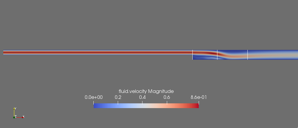
steady=true2.2.2. Flow visualization
The solution obtained by ParaView is represented in the figure below,it is a final solution obtained in a stationary state:
2.2.3. Comparaison between simulated and theorical results:
To visualize the flow profile we pass to the graphical representation of the simulated results using plotly bibliography, then we will compare the results obtained in the simulation for Re=389 with the results of the literature.
Simulated results:
The graph below show as the flow profile simulated at the different vertical lines \(x_r/S\):
Comparaison
The graph below show the comparison of the theorical solution with simulate flow solution for:
-
\(x/S=0.0\):
-
\(x/S=5.41\):
-
\(x/S=11.84\):
Based on the results obtained during the simulation and the theoretical results we calculate the Root Mean Square Error(RMSE) for each case, the results are grouped in the table below:
| \(x/S\) | RMSE | Observation average | Model variance |
|---|---|---|---|
0.0 |
3.63 |
44.47 |
8.16 % |
5.41 |
8.54 |
24.34 |
35.08 % |
11.84 |
8.86 |
25.31 |
35 % |
Indeed, according to the results the variance of the model for \(x/S=0.0\), \(x/S=5.41\) and \(x/S=11.84\) corresponds to only 8.16%, 35.08% and 35.00% of the mean of the observations respectively, we can therefore say that the model has a high variance at \(x/S=5.41\) and \(x/S=11.84\) contrary at \(x/S=0.0\) the variance is low.
2.3. Results for Re=1095
To have a stationary solution when Re=1095 the problem has to be treated in an unstationary frame.
| In this case the solution will depend on time. |
2.3.1. Configuration files
json file
{
    "Name": "Laminar, Isothermal Backward Facing Step Benchmark",
    "ShortName":"ecoulementstationnaire",
    "Models":
    {
        "equations":"Navier-Stokes"
    },
    "Parameters":
    {
        "h":"5.2e-3",
        "s":"4.9e-3",
        "uave":"1.5322"
    },
    "Materials":
    {
        "omega":
        {
            "rho":"1.23",
            "mu":"1.79e-5"
        }
    },
    "BoundaryConditions":
    {
        "velocity":
        {
            "Dirichlet":
            {
                "inlet":
                {
                    "expr":"{6*uave*((y-s)/h)*(1-((y-s)/h)),0}:uave:s:h:y"
                },
                "wall1":
                {
                    "expr":"{0,0}"
                },
                "wall2":
                {
                    "expr":"{0,0}"
                },
                "wall3":
                {
                    "expr":"{0,0}"
                }
            }

        },
        "fluid":
        {
            "outlet":
            {
                "outlet":
                {
                    "expr":"0"
                }
            }
        }
    },
    "PostProcess":
    {
        "Exports":
        {
            "fields":["velocity"]
        }
    }
}
cfg file
directory=resulats/instationnaire1095/P1
[case]
discretization= P2P1G1
dimension=2
[fluid]
filename=$cfgdir/laminar.json
mesh.filename=$cfgdir/lami.geo
gmsh.hsize=0.0005
solver= Newton #Oseen #Newton #Picard,Newton
linearsystem-cst-update=false
jacobian-linear-update=false
snes-monitor=true
pc-type= gams #gasm,lu
[fluid.bdf]
order=2
[ts]
time-step=0.1
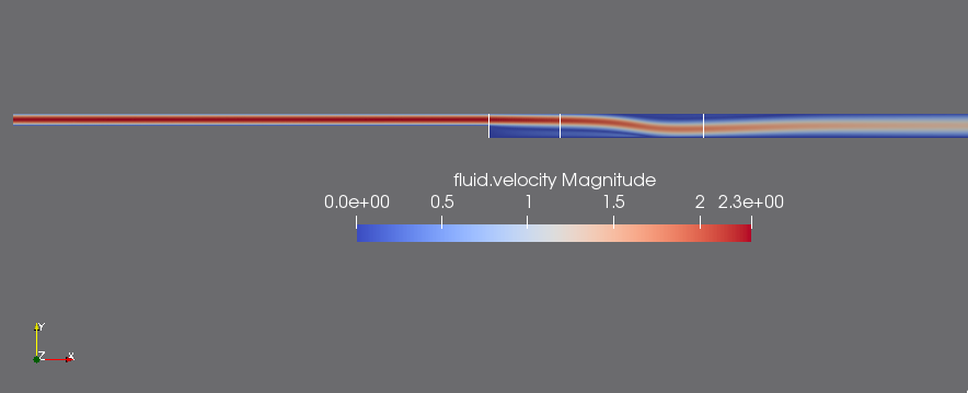
time-final=52.3.2. Flow visualization
The solution obtained by ParaView is represented in the figure below,it is a final solution obtained in a stationary state:
Comparaison between simulated and theorical results:
To visualize the flow profile we pass to the graphical representation of the simulated results using plotly bibliography, then we will compare the results obtained in the simulation for Re=1095 with the results of the literature.
Simulated results:
The graph below show as the flow profile simulated at the different vertical lines \(x/S\):
Comparaison
The graph below show the comparison of the theorical solution with simulate flow solution for:
-
\(x/S=0.0\):
-
\(x/S=7.04\):
-
\(x/S=19.04\):
Based on the results obtained during the simulation and the theoretical results we calculate the Root Mean Square Error(RMSE) for each case, the results are grouped in the table below:
| \(x/S\) | RMSE | Observation average | Model variance |
|---|---|---|---|
0.0 |
9.33 |
134.03 |
6.96 % |
7.04 |
10.05 |
67.86 |
14.80 % |
19.04 |
12.03 |
57.79 |
20.81 % |
Indeed, according to the results the variance of the model for \(x/S=0.0\), \(x/S=7.04\) and \(x/S=19.04\) corresponds to only 6.96%, 14.80% and 20.81% of the mean of the observations respectively, so we can say that the model has a low variance.
2.4. Reattachment length in the laminar flow regime
To illustrate the relation between \(x_r/S\) and the Rynolde number we have performed several simulations at different Re, such as \(x_r\) is the recirculation zone.
| \(x_r/S\) | Rynolds |
|---|---|
2.04 |
50 |
3.5 |
150 |
4.5 |
200 |
5.3 |
250 |
6.20 |
300 |
6.60 |
350 |
For the different Reynolds values mentioned in the table[5] the flow is stationary and the length of the simulated recirculation zone increases fairly linearly with Re.