Mesh extraction with LevelSet

Such as the extraction with polygons, the levelSet is one method we explored to errase problematic areas. Its main interest is that it is almost automatic, after the circles are placed.

1. Method

By using a scalar function named \(\phi\) define as null value is obtained when it reach an interface of two domains.

We denote \(\Omega_1\) and \(\Omega_2\) two domains with \(\Gamma\) the interface betwen them. Then \(\phi\) can be define as

\[\phi(\boldsymbol{x}) = \left\{ \begin{array}{cccc} \text{dist}(\boldsymbol{x}, \Gamma), & \boldsymbol{x}& \in &\Omega_1 \\ 0, & \boldsymbol{x}& \in &\Gamma\\ -\text{dist}(\boldsymbol{x}, \Gamma), & \boldsymbol{x}& \in & \Omega_2 \end{array} \right.\]

with \(\text{dist}(\boldsymbol{x}, \Gamma ) = \underset{\boldsymbol{y} \; \in \; \Gamma}{\min}( |\boldsymbol{x} - \boldsymbol{y}| ).\)

This function \(\phi\) had also the following property \(|\nabla\phi|=1\).

Moreover, the unit normal vector \(\boldsymbol{n}\) outgoing from the interface and the curvature \(\mathcal{\kappa}\) can be obtained from the levelset function.

\[\boldsymbol{n}=\frac{\nabla\phi}{|\nabla\phi} \\ \mathcal{\kappa}=\nabla \cdot \boldsymbol{n}= \nabla \cdot \frac{\nabla\phi}{|\nabla\phi|}\]

Now we have exposed the levelset function, we need to define how the levelset will evolve and will spread into all the space. To do this, we use the following advection equation :

\[\partial_t\phi+\boldsymbol{u}\cdot\nabla\phi=0\]

where \(\boldsymbol{u}\) is an incompressible velocity field.

1.1. Heaviside and Dirac functions

We define also the regularized Heaviside function

\[H_\varepsilon(\phi) = \left\{ \begin{array}{cc} 0, & \phi \leq - \varepsilon,\\ \dfrac{1}{2} \left(1+\dfrac{\phi}{\varepsilon}+\dfrac{\sin\left(\dfrac{\pi \phi}{\varepsilon}\right)}{\pi}\right), & -\varepsilon \leq \phi \leq \varepsilon, \\ 1, & \phi \geq \varepsilon \end{array} \right.\]

and the regularized Dirac function

\[\delta_\varepsilon(\phi) = \left\{ \begin{array}{cc} 0, & \phi \leq - \varepsilon,\\ \displaystyle\dfrac{1}{2 \varepsilon} \left(1+\cos\left(\dfrac{\pi \phi}{\varepsilon}\right)\right), & -\varepsilon \leq \phi \leq \varepsilon, \\ 0, & \phi \geq \varepsilon. \end{array} \right.\]

The first one gives a different value to each side of the interface ( here 0 in and 1 out ). The second one allow us to define quantities, with value different from 0 at the interface. A typical value of \(\varepsilon\) in literature is \(1.5h\) where \(h\) is the mesh step size.

It should be noted that these functions allow us to determine respectively the volume and the surface of the interface by

\[V^+_{\varepsilon} = \int_{\Omega} H_\varepsilon \\ S^{\Gamma}_{\varepsilon} = \int_{\Omega} \delta_\varepsilon\]

2. Implementation

As write ahead, we will use circles as our method \(\phi\), describe in a text file

auto Vh = Pch<1> (mesh) ;
std::ifstream flux(soption(_name="circles")) ;
    std::ostringstream ostr;
    int nbCircles ;
    flux >> nbCircles ;

    for (int i = 0 ; i < nbCircles ; i ++) {
        flux >> x_center ;
        flux >> y_center ;
        ostr << "((x-" << x_center*pixelsize << ")^2+(y-" << y_center*pixelsize << ")^2-" << radius*radius << ")" ;
        if (i != nbCircles-1)
            ostr << "*" ;
    }

    ostr << ":x:y";
    auto phi = Vh->element( expr( ostr.str() ) );

We also build Heaviside and Dirac functions

auto H = vf::project(_space=Vh, _range=elements(mesh),_expr=
                chi( idv(phi) < cst(-epsilon) ) * 0.
              + chi( idv(phi) >= cst(-epsilon) )
              * chi( idv(phi) <= cst(epsilon) )
              * 1./2*(1+idv(phi)/cst(epsilon) + sin(pi*idv(phi)/cst(epsilon))/pi)
              + chi (idv(phi) > cst(epsilon) ) * 1. ) ;
        toc("Heaviside") ;
        e->step(current_time)->add("H", H) ;

        tic() ;
auto D = vf::project(_space=Vh, _range=elements(mesh),_expr=
                chi( idv(phi) < cst(-epsilon) ) * 0.
              + chi( idv(phi) >= cst(-epsilon) )
              * chi( idv(phi) <= cst(epsilon) )
              * 1./(2.*cst(epsilon))*(1.+cos(pi*idv(phi)/cst(epsilon)))
              + chi (idv(phi) > cst(epsilon) ) * 0. ) ;
        toc("Dirac") ;
        e->step(current_time)->add("D", D) ;

Then we want to extend our \(\phi\) function with ExtenderFromInterface<2,1, Hypercube> efi(Vh, phi) object from Feel++.

        auto beta = ((1.-betab*beta_part-gamma*gamma_part)/(1.+alpha*sqrt(inner(gradv(px),(gradv(px)))))) * (trans(gradv(phi))/sqrt(inner(gradv(phi),gradv(phi)))) ;

        efi.update(phi) ;
        auto beta_x = Vh->element () ;
        auto beta_y = Vh->element () ;
        beta_x.on(_range=elements(mesh), _expr=beta(0,0)) ;
        beta_y.on(_range=elements(mesh), _expr=beta(1,0)) ;
        efi.extendFromInterface(beta_x) ;
        efi.extendFromInterface(beta_y) ;
        beta_p.on(_range=elements(mesh), _expr=vec(idv(beta_x), idv(beta_y))) ;

        beta_p.on(_range=elements(mesh), _expr=idv(beta_p)*chi(sqrt(inner(trans(idv(beta_p)), trans(idv(beta_p)))) > cst(umin))) ;

We define finally the composent of the advection problem in order to describe and then solve it.

tic() ;
        auto supg_term = inner(grad(psi), trans(idv(beta_p))) ;
        toc("supg_term") ;

        tic() ;
        auto L_op = inner(gradt(phi), trans(idv(beta_p))) + sigma*idt(phi);
        toc("L_op") ;

        tic() ;
        auto tau_supg = h() / max (2.*sqrt(inner(idv(beta_p), idv(beta_p))), umin*umin);
        toc("tau_supg") ;


        tic() ;
        l = integrate(_range=elements(mesh),
                _expr=f*id(psi));
        l += integrate(_range=elements(mesh),
                _expr=tau_supg*supg_term*f);
        toc("form1") ;

        tic() ;
        a = integrate( _range=elements(mesh),
                _expr=(sigma*idt(phi)+inner(trans(idv(beta_p)),gradt(phi)))*id(psi));
        a += integrate (_range=elements(mesh),
                _expr=tau_supg*supg_term *L_op);
        toc("form2") ;

        tic() ;
        a.solve(_rhs=l, _solution=phi) ;
        toc("solve") ;

After solve this, we update \(\phi\) and we repeat this operation until one of the stop conditions is reach.

 phi = thefms->march(phi) ;
 } while ( mean_beta_x > tolerance || mean_beta_y > tolerance || erreurL2 > tolerance) ;

We can also, at the end of the program, extract the mesh without ( or with only ) the areas inside \(\phi\)

auto marker = vf::project (Xh0, elements(mesh), chi(idv(phi) <= cst(0.)));
        //: vf::project(Xh0, elements(mesh), chi(idv(polygon) > cst(0.))) ;
    mesh ->updateMarker2(marker) ;
    auto submesh = createSubmesh(mesh, marked2elements(mesh,doption("parameters.a"))) ;
    saveGMSHMesh(submesh,"levelSetmesh.msh");

3. Results

The levelset is now operational with our slopes areas problems ( with a Gaussian filter on the data ) as the pictures below explain it

Levelset

levelSet

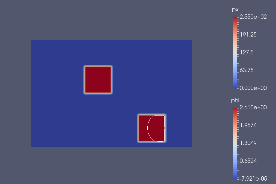
However, we encounter some difficulties to pair it with our specific mesh construction and to parallelize it, coupled with the project time limit.