Serial control benchmark
This part will be dedicate to the benchmarking of the serial control application, that resolve our problem for \mathbf{N} set of data.
The default data we will be using here are as follows :
-
Image size : 1280*960
-
Number of processors : 4
-
Number of case : 4 ( only for serial_control )
All the test are realised with the ML preconditionner, on the Irma Atlas Cluster.
1. Reminder
In the case of the serial control application, we would like to pass trough multiple sets of slope datas, with the same principal aspect, such as image size or area of interest.
The program can be decomposed into main parts :
-
The initial initialization
-
Mesh correspond at the time need to build the mesh ( nodes and elements ) and prepare it to use.
-
auto mesh = boost::make_shared<MeshStructured>( ioption("Scala")*(x.rows()),
                                                ioption("Scala")*(x.cols()),
                                                doption(_name="pixelsize"),
                                                Environment::worldComm() );
mesh->components().reset();
mesh->components().set( size_type(MESH_UPDATE_ELEMENTS_ADJACENCY|MESH_NO_UPDATE_MEASURES) );
mesh->updateForUse();-
Vh is the part where we built the function space, used for defining elements ( test and trial ).
auto Vh = Pch<1> ( mesh ) ;-
Elements is the build of the trial and test elements, as well that we will browse trough the mesh, as well as "data" elements, which will help us to define our problem.
auto u = Vh->element () ;
auto v = Vh->element () ;
auto px = Vh->element () ;
auto py = Vh->element () ;-
HbfToFeel is the time to build the object that will allow us to transfer the data from the hbf files into our "data" elements.
Hbf2FeelppStruc h2f( nx, ny, Vh );-
lhs is the build of the left ( bilinear ) side of our equation problem.
auto a = form2( _trial=Vh, _test=Vh);
a = integrate( _range=elements(mesh),
_expr=gradt(u)*trans(grad(v)));-
The loop ( A complete loop is reffered as Set )
-
rhs is the build of the right ( bilinear ) side of our equation problem.
-
x = readHBF( Environment::expand("${holo3_srcdir}/data/surface_reconstruction/input/Issue1/Surface_Basis/Dxsurface"+std::to_string(i)+".hbf") );

y = readHBF( Environment::expand("${holo3_srcdir}/data/surface_reconstruction/input/Issue1/Surface_Basis/Dysurface"+std::to_string(i)+".hbf") );

px = h2f( x, px );
py = h2f( y, py );

auto l= form1( _test=Vh );
l = integrate(_range=elements(mesh),
_expr=grad(v)*vec(idv(px),idv(py)));-
The solver part is the time need to solve our equation , with possible conditions to take in account.
a.solve(_rhs=l,_solution=u,_post=zeromean)1.1. Processor numbers scalability
Just like the previous application, we want to determine here how the time consumption will evolve when the number of processor used or the size of the images will change, but also, in this particular case, with the number of image set ( aka case ) the application must resolve.
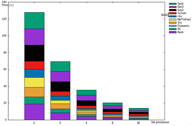
To resolve four cases in a row, we pass to 140 s in sequential to approximatly 20 s with 16 processors.
1.2. Image size scalability
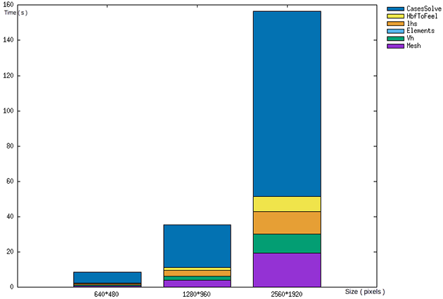
Just as the first program, time react as exepected when slope data size is increased.

For the weak scalability, we retrieve the same pattern as before. The first two test are pretty similar and the difference is so slim. However at the third case, time increase again drastically.
NOTE : For the third case, the program cannot finish to solve all the case ( four ) at the moment. The time of cases solve is so appraoch from time data we have ( firsts solve completed )
1.3. Case number scalability
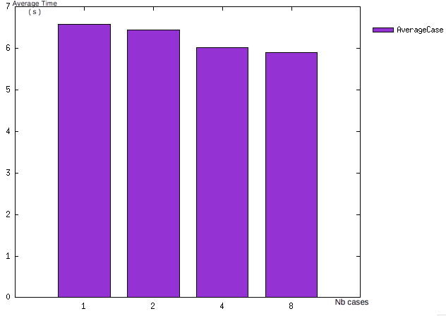
We saw here that, with four processors, we have an average time equals to 7s for resolve one case.
The average time need for one case, aka one set of data and the resolution, don’t change whatever number of cases wanted, without taking in consideration possible other actions on processors.