Methodology
1. Tangent Vectors to Parametrized Surfaces
Suppose that \(\Phi\) is a parametrized surface that is differentiable at \(\left(u_{0}, v_{0}\right) \in \mathbb{R}^{2}\).
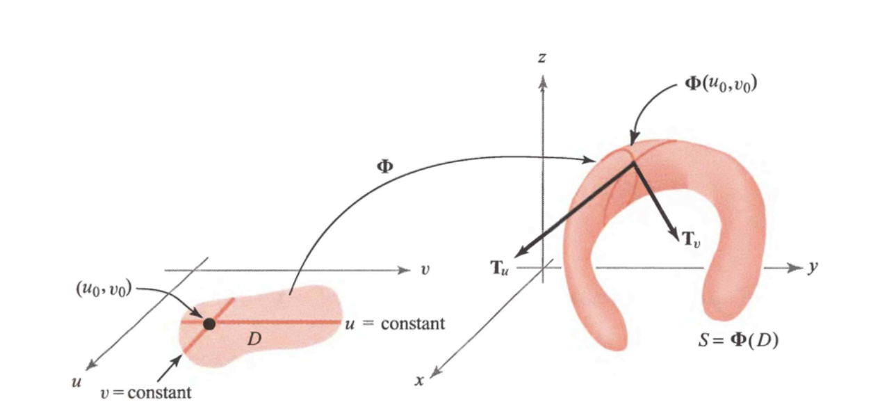
Fixing \(u\) at \(u_{0},\) we get a \(\operatorname{map} \mathbb{R} \rightarrow \mathbb{R}^{3}\) given by \(t \mapsto \boldsymbol{\Phi}\left(u_{0}, t\right),\) whose image is a curve on the surface.
the vector tangent to this curve at the point \(\Phi\left(u_{0}, v_{0}\right),\) which we denote by \(\mathbf{T}_{v},\) is given by
Similarly, if we fix \(v\) and consider the curve \(t \mapsto \Phi\left(t, v_{0}\right),\) we obtain the tangent vector to this curve at \(\Phi\left(u_{0}, v_{0}\right),\) given by
We can use the fact that \(\mathbf{n}=\mathbf{T}_{u} \times \mathbf{T}_{v}\) is normal to the surface to both formally define the tangent plane and to compute it.
DEFINITION: The Tangent Plane to a Surface
If a parametrized surface \(\boldsymbol{\Phi}: D \subset \mathbb{R}^{2} \rightarrow \mathbb{R}^{3}\) is regular at \(\Phi\left(u_{0}, v_{0}\right),\) that is, if \(\mathbf{T}_{u} \times \mathbf{T}_{v} \neq \mathbf{0}\) at \(\left(u_{0}, v_{0}\right),\) we define the tangent plane of the surface at \(\Phi\left(u_{0}, v_{0}\right)\) to be the plane determined by the vectors \(\mathbf{T}_{u}\) and \(\mathbf{T}_{v} .\) Thus, \(\mathbf{n}=\mathbf{T}_{u} \times \mathbf{T}_{v}\) is a normal vector, and an equation of the tangent plane at \(\left(x_{0}, y_{0}, z_{0}\right)\) on the surface is given by
where \(\mathbf{n}\) is evaluated at \(\left(u_{0}, v_{0}\right) ;\) that is, the tangent plane is the set of \((x, y, z)\) satisfying \((1) .\) If \(\mathbf{n}=\left(n_{1}, n_{2}, n_{3}\right)=n_{1} \mathbf{i}+n_{2} \mathbf{j}+n_{3} \mathbf{k},\) then formula (1) becomes
Suppose a surface \(S\) is the graph of a differentiable function \(g: \mathbb{R}^{2} \rightarrow \mathbb{R} .\)
We wish to write \(S\) in parametric form and show that the surface is smooth at all points \(\left(u_{0}, v_{0}, g\left(u_{0}, v_{0}\right)\right) \in \mathbb{R}^{3}\)
We write \(S\) in parametric form as follows:
which is the same as \(z=g(x, y) .\) Then at the point \(\left(u_{0}, v_{0}\right)\)
and for \(\left(u_{0}, v_{0}\right) \in \mathbb{R}^{2}\)
This is nonzero because the coefficient of \(\mathbf{k}\) is \(1\) ; consequently, the parametrization \((u, v) \mapsto(u, v, g(u, v))\) is regular at all points.
The tangent plane at the point \(\left(x_{0}, y_{0}, z_{0}\right)=\left(u_{0}, v_{0}, g\left(u_{0}, v_{0}\right)\right)\) is given, by formula \((1),\) as
where the partial derivatives are evaluated at \(\left(u_{0}, v_{0}\right) .\)
|
Remembering that \(x=u\) and \(y=v,\) we can write this as
\[z-z_{0}=\left(\frac{\partial g}{\partial x}\right)\left(x-x_{0}\right)+\left(\frac{\partial g}{\partial y}\right)\left(y-y_{0}\right)\]
where \(\partial g / \partial x\) and \(\partial g / \partial y\) are evaluated at \(\left(x_{0}, y_{0}\right)\) |
2. Reconstruction from slope data
In this docummentation, we study a method for numerical integration of a gradient field over a 2 D-grid. Our aim is to estimate the values of a function \(z: \mathbb{R}^{2} \rightarrow \mathbb{R},\) over a set \(\Omega \subset \mathbb{R}^{2}(\text { reconstruction domain })\) where an estimate \(\mathbf{d}=\) \([p, q]^{\top}: \Omega \rightarrow \mathbb{R}^{2}\) of its gradient \(\nabla z\) is available.
We aim at the following properties:
-
\(\mathcal{P}_{\text {Fast }}:\) be as fast as possible;
-
\(\mathcal{P}_{\text {Robust }}:\) be robust to a noisy gradient field;
-
\(\mathcal{P}_{\text {FreeB }}:\) be able to handle a free boundary;
-
\(\mathcal{P}_{\text {NoRect }}:\) be able to work on a non-rectangular domain \(\Omega\)
-
\(\mathcal{P}_{\text {NoPar: have }}\) no critical parameter to tune.
Formally, we want to solve the following equation in the unknown depth \(\operatorname{map} z\)
A natural way to deal with this problem is to write as an optimization problem using quadratic regularization, this amounts to minimizing the following functional:
where \(\Omega \subset \mathbb{R}^{2}\) denotes the domain ofintegration, and \(\mathbf{d}=[p, q\)] is the datum of the problem, which we call the gradient field.
This functional is strictly convex in \(\nabla z,\) but it does not admit a unique minimizer \(z^{*}\) since, for any constant \(K \in \mathbb{R}, \mathcal{F}_{L_{2}}\left(z^{*}+K\right)=\mathcal{F}_{L_{2}}\left(z^{*}\right)\)
The minimization of \(\mathcal{F}_{L_{2}}(z)\) requires that the associated Euler-Lagrange equation is satisfied.
i.e. \(\frac{\partial\mathcal{L}}{\partial z} - \frac{\partial}{\partial u}(\frac{\partial \mathcal{L}}{\partial z_p}) - \frac{\partial}{\partial v}(\frac{\partial\mathcal{L}}{\partial z_q})= 0 \) where \(\mathcal{L} = \|\nabla z(u,v) - d(u,v)\|^2\) and \(\nabla z = (z_p, z_q)^t\)
so we get the following condition :
Which is an equation we know how to solve, the Poisson equation.
Solving this equation is not a sufficient condition for minimizing \(\mathcal{F}_{L_{2}}(z),\) but this is the case if either \(z\) (Dirichlet) or \(\nabla z(\text { Neumann })\) is known on the boundary \(\partial \Omega\) of \(\Omega\)
In the absence of such boundary condition, the so-called natural boundary condition, which is of the Neumann type, must be considered. In the case of \(\mathcal{F}_{L_{2}}(z)\) this boundary condition is written:
where \(\boldsymbol{\eta}\) is the outer unit normal to the boundary \(\partial \Omega\) in the image plane.