HiFiMagnet Salome Plugin

Welcome to HiFiMagnet Salome Plugin documentation!

The HiFiMagnet Salome Plugin documentation describes its installation, its features, its uses and provides some references.

If you find errors or omissions in this document, please don’t hesitate to submit an issue or open a pull request with a fix. We also encourage you to ask questions and discuss any aspects of the project on the HiFiMagnet Gitter forum. New contributors are always welcome!

Introduction

The HiFiMagnet Salome Plugin allows to easily:

define CAD geometry for Solenoidal High Field Magnet
mesh these geometries.

In a near future, the plugin will also provides tools:

to define files required for running simulations,
to run calculations either locally or remotely,
to analyze the results

The meshing features require a license to MeshGems suite.

Quick Starts

This document will illustrate how to simply use HiFiMagnet Salome plugin and give examples for most common operations.

Custom installation, eg. for native installation, is detailed in the dev section.

1. Getting HiFiMagnet Salome plugin

They are several way to use HiFiMagnet Salome plugin. The easiest way is to use container, either Docker based or Singularity based. If your system support singularity containers we recommend to use them instead of Docker ones.

1.1. from sregistry

To get the Salome singularity image you need first to get you token on a valid sregistry:

connect to the Sregistry service (eg cesga sregistry use the FiWare authentification}
in the top right scrolling menu with your user id, select Token
copy the line to a .sregistry in your home directory

Then from a terminal:

export SREGISTRY_CLIENT=registry
export SREGISTRY_CLIENT_SECRETS=~/.sregistry-cesga
[export SREGISTRY_STORAGE=...]

sregistry pull --name salome-8.4.0.simg hifimagnet/salome:8.4.0

The singularity image will be downloaded to a file name: hifimagnet-salome-8.4.0.simg.

SREGISTRY_STORAGE enables you to specify a directory to hold the singularity images. By default images will be downloaded to $HOME/.sregistry

On some systems (eg without NVidia graphic video card), it may be more convenient to use hifimagnet/salome-mesa:8.4.0 image instead of the standard one. See here for details.

1.2. from dockerhub

You need to be member of Feel++ team on dockerhub to be able to download the image. To get the image:

docker login
docker pull feelpp/salome:8.4.0-nvidia

Check the existing docker images on feelpp/salome dockerhub

Supported Salome versions are: 8.3.0, 8.4.0 and 8.5.0.
If you do no need HiFiMagnet Salome plugin you can use a public version of Salome docker image that you may find in dockerhub.

To use Salome in GUI mode the docker container should contain appropriate graphics drivers. Actually only nvidia graphic cards are supported. To custom the images for you graphics card you should have a look at the scripts generating the images.

For system without Nvidia graphic card, we recommend to fellpp/salome:8.4.0-mesa instead

1.3. Install from Lncmi Salome_Packages

You can also download the binaries for you platform and the corresponding installation script. Supported platforms are:

Debian/Stretch
Ubuntu/Xenial (aka 16.04 LST)

On Windows 10 Pro with WSL enabled, you can also follow this procedure to install HiFiMagnet Salome plugin. Before running just install a X11 server. We recommend MobaXterm 10.9 or latter.

2. Running HiFiMagnet Salome plugin

HiFiMagnet Salome plugin can be run either in GUI or TUI mode. TUI stands for Terminal User Interface.

To switch to TUI mode, use -t option. Add -b option to the use TUI in batch mode.

2.1. from Singularity container

Assuming we use salome.simg singularity image:

singularity exec [--nv] \
  -H $HOME:/home/$USER \
  -B $STORE/Distene/:/opt/DISTENE/DLim \
  salome.simg \
  salome [-t -b] ...

Note the --nv flag is mandatory to run in GUI mode and is only supported by nvidia drivers.

2.2. from Docker container

xhost local:root
docker run -ti --rm -e DISPLAY \
   --net=host --pid=host --ipc=host \
   --env QT_X11_NO_MITSHM=1 \
   -v /tmp/.X11-unix:/tmp/.X11-unix \
   -v $HOME/.Xauthority:/home/feelpp/.Xauthority \
   -v /opt/DISTENE/DLim:/opt/DISTENE/DLim \
   feelpp/salome:8.4.0-nvidia salome [-t -b] ...

On Windows:

Start MobaXterm (that provides a running X11 server)
Then run:

docker run -it --rm -e DISPLAY :0 feelpp/salome:8.4.0-nvidia

On MacOs X:

start XQuartz
In XQuartz: defaults write org.macosforge.xquartz.X11 enable_iglx -bool true
Restart XQuartz
Then run:

ip=$(ifconfig en0 | grep inet | awk '$1=="inet" {print $2}')
xhost +$ip
docker run -it --rm -e DISPLAY $ip:0 feelpp/salome-8.4.0:nvidia

You may need to adapt the line to get the working ip of your machine depending on your internet connection.

See this presentation for details

2.3. Main commands

We will omit the part of the command related to the use of Singularity or Docker to only give the Salome command. If you plan to run these commands from a Singularity or Docker image, just start the container (see here, watch out to not forget to enable the display if you want to use the GUI mode).

Examples files may be found here.

The structure of the yaml file describing the geometry and mesh be generated will be described in the data structure section.

Generation of an Insert with an air box in TUI mode

salome [-m GEOM,SMESH,HIFIMAGNET] [-t -b] \
   ${HIFIMAGNET}/HIFIMAGNET_Cmd.py \
   args:--cfg=Insert-H1H4-Leads-2t.yaml[,--air[,--infty_Rratio=2,--infty_ZRatio=1.5],--mesh]

$HiFiMagnet is the install directory of HiFiMagnet Salome plugin, eg /opt/SALOME-8.4.0-Debian-DB9.5/BINARIES-DB9.5/HIFIMAGNET/bin/salome.

A 4 helix insert with sourring air (in transparent red)

Insert-H1H4-Leads-2t.yaml can be found in /usr/local/share/salome/H1H4 in singularity images.

2.4. On Remote desktop

copy MeshGems licence file on your account in the Visu resource in ${LICDIR} directory
pull Salome HiFiMagnet image with Mesa support from Sregistry.

export SREGISTRY_CLIENT=registry
export SREGISTRY_CLIENT_SECRETS=$HOME/.sregistry
export SREGISTRY_STORAGE=$LUSTRE/singularity_images
module load singularity
singularity run -B /mnt shub://sregistry.srv.cesga.es/mso4sc/sregistry --quiet pull hifimagnet/salome-mesa:8.4.0

Then to run Salome type:

module load singularity
singularity run --nv -B ${LICDIR}:/opt/DISTENE/DLim:ro --app salome ${SREGISTRY_STORAGE}/hifimagnet-salome-mesa-8.4.0.simg

You can also start the container:

singularity exec -B ${LICDIR}:/opt/DISTENE/DLim:ro -${SREGISTRY_STORAGE}/hifimagnet-salome-mesa-8.4.0.simg

and run type the following command within the container:

GALLIUM_DRIVER=llvmpipe salome

Alternatively you can also use run_salome.sh:

./run_salome.sh -l ${LICDIR} [-i [${SREGISTRY_STORAGE}/]hifimagnet-salome-mesa-8.4.0.simg]

Data Structure

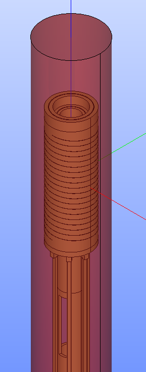
An insert consists in a set of:

helices,
connection rings

and eventually an inner and an outer currentLead.

Each structure is defined as a yaml file.

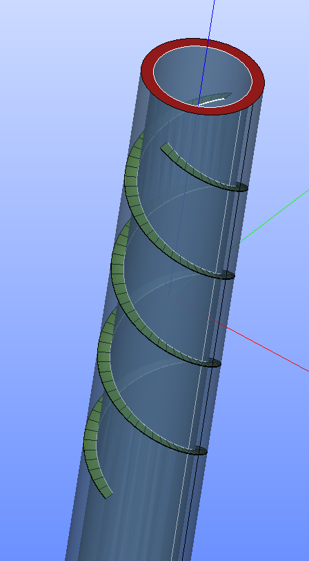
1. helix structure

An helix is actually a cylindrical tube which exhibit a single or double helical cut made by EDM. The path of the helical cut is provided in a separate file *_cut_salome.dat.

!<Helix>
name: HL-31_H1, (1)
dble: true, (2)
odd: true, (3)
r:, (4)
  - 19.3
  - 24.2
z:, (5)
  - -226
  - 108
cutwidth: 0.22, (6)
axi: !<ModelAxi>, (7)
  ...
m3d: !<Model3D>, (8)
  ...
shape: !<Shape>, (9)
  ...

1	name of the CAD to be created (it corresponds to the name in the Lncmi Bureau d’Etudes nomemclature).
2	specify if the helix is single or double (ie. helical cut).
3	specify if the helix is odd or even (the helical cut patch orientation changes from one helix to the other).
4	the radial dimension in mm.
5	the axial dimension in mm.
6	the width of the helical cut.
7	the corresponding axi model.
8	the ………… 3d model.
9	definition of the shape added along the helical path

1.1. `axi` structure

The axi structure defines the helical cut along with the file *_cut_salome.dat

axi: !<ModelAxi>
  name: "HL-31.d", (1)
  h: 86.51, (2)
  pitch:, (3)
    - 17.302
  turns:, (4)
    - 10

1	name of the axisymetrical description of the magnet (see magnettools)
2	half electrical length; $2h$ corresponds to the axial length of the helical path centered on the origin.
3	list of pitch $p_i$
4	list of turns $n_i$

The helical path consists in a set of $i$ helices with a pitch $p_i$ and a number of turns $n_i$

1.2. `m3d` structure

m3d: !<Model3D>
  cad: "HL-31-202MC", (1)
  with_shapes: false, (2)
  with_channels: false, (3)

1	name of the CAD geometry (usually stems from the Bureau d’Etudes nomemclature to keep track of the CADs)
2	indicates wether shapes are added or not on the helical path
3	indicates wether micro-cooling channels are added (only for radial helices)

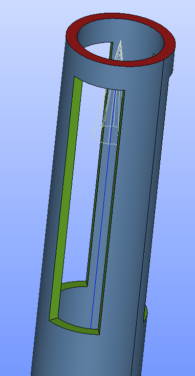
1.3. `shape` structure

shape: !<Shape>
  name:, (1)
  profile: "", (2)
  length: 0, (3)
  angle: 0, (4)
  onturns: 0, (5)
  position: ABOVE, (6)

1	name of the shape to be added (actually it’s the name of the shape file description without extension )
2	name of CAD profile (this name comes from the Bureau d’Etudes nomemclature to keep track of the CADs)
3	angular length of the shape in degree
4	angular shift between 2 consecutive shapes (optionnal)
5	specify on wich turns the shape are disposed
6	orientation of the shape (values valid are …)

The shape file description is a simple .dat file that defines the number of points of the shape and theirs coordinates in a local cartesian frame:

#Shape : HL-31-985 pour H14
#N_i
20
#X_i F_i
-3.75	0
...
 3.75	0

1.4. `helical cut` structure

The geometry of the helical cut is computed using MagnetTools. It provides the coordinates of the cut in developed form which will be mapped onto the outer cylinder boundary of an helix.

# Fichier de decoupe Salome V7.3.0, (1)
# Fichier d'Optimisation [Aubert] : HL-31_H1_.d
# author: trophime
# date : Tue Sep 30 13:32:59 2014
#
# Orientation : gauche

#theta[rad] 	Shape_id[]	Z[mm], (2)
#
-0.00000000e+00	           0	8.65100000e+01
-1.83673270e+00	           0	7.78590000e+01
...
-5.15703414e+01	           0	-7.78590000e+01
-5.34070738e+01	           0	-8.65100000e+01

1	header
2	`theta`, `Z_i` defines the coordinates of the point in a 2D cartesian frame (note: $\text{theta} \in [0,2\pi*n_{turns}$] with $n_{turns}$ the total number of turn of the path) and `Shape_id` indicates the precense or absence of shape and eventually of micro-cooling channel

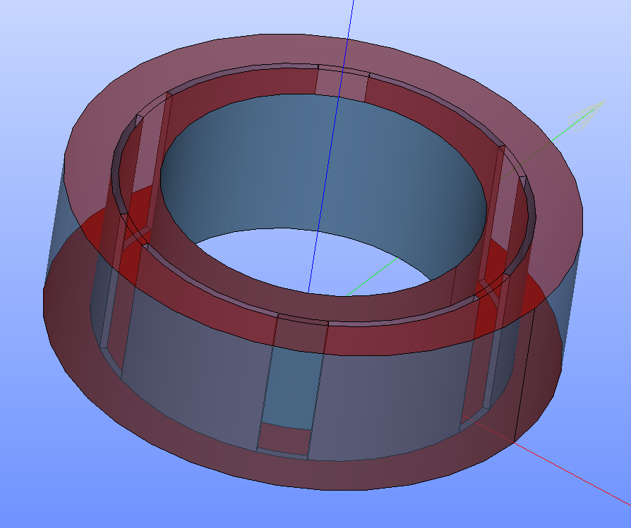
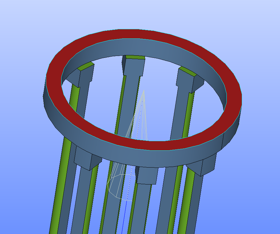
ring

A ring ensure the electrical and mechanical connection between 2 consecutive helices. It is a cylinder eventually with $n$ cylindrical slots, disposed at regular angular interval $angle$ in it to ensure a proper cooling of the connected helices.

!<Ring>
name: Ring-H1H2, (1)
BPside: true, (2)
r: [19.3, 24.2, 25.1, 30.7], (3)
z: [0, 20], (4)
fillets: false, (5)
n: 6
angle: 46

1	name of the CAD to be created (it corresponds to the name in the Lncmi Bureau d’Etudes nomemclature).
2	specifiy the position of the ring: either on Low pressure (eg `BPside=true`) or High Pressure side (eg `BPside=false`)
3	the radial dimension in mm.
4	the axial dimension in mm.
5	indicates the presence or the absence of cylindrical slot

1. CurrentLeads

1.1. Inner Lead

!<InnerCurrentLead>
fillet: 0
f: 480.0
foles: [123, 12, 90, 60, 45, 3]
name: Inner
r: [19.3, 24.2]

1.2. Outer Lead

!<OuterCurrentLead>
bar: [4, 9, 5, 501]
h: 10
support: [10, 5, 40, 45]
name: Outer
r: [19.3, 24.2]

2. insert

!<Insert>
name: "HL-31", (1)
Helices:, (2)
  - HL-31_H1
  ...
Rings:, (3)
  - Ring-H1H2
  ...
CurrentLeads:, (4)
  - inner
  - outer-H14
innerbore: 18.54, (5)
outerbore: 186.25, (6)
HAngles:, (7)
RAngles:, (8)

1	name of the CAD geometry
2	list of helices
3	list of rings
4	define inner and outer current leads
5	radius of the inner bore tube
6	radius of the external tube holding the helices insert
7	angular orientation of helices (optionnal)
8	angular orientation of rings (optionnal)

3. mesh

The mesh is generated from the command line when the option --mesh is passed to salome. The first time the mesh is generated, a file , namely Insert_meshdata.yaml where Insert.yaml is the actual yaml cfg file used in the main command line, is also created containing main mesh parameters. This file may be later used to regenerate the same mesh or modify to get a finner or coarser mesh.

So far only MeshGems mesher is supported.

Here is an example of the yaml cfg file:

!<MeshData>
geometry: BancMesure_H3H4, (1)
name: BancMesure_H3H4-air, (2)
algosurf: BLSURF, (3)
algovol: GHS3D, (4)
Gradation: 1.05, (5)
KeepFiles: 0, (6)
MakeGroupsOfDomains: 0, (7)
OptimizationLevel: 4, (8)
RemoveLogOnSuccess: 1, (9)
MaximumMemory: 450559, (10)
surfhypoths:, (11)
- - - HL-31_H3_inputs
    - [2, 1, 2.16, 0.65, 65.0, 1.546]
  - - HL-31_H3_boundary
    - [2, 1, 2.16, 0.65, 65.0, 1.546]
  - - HL-31_H3_interface
    - [2, 1, 0.72, 0.065, 6.5, 0.1546]
  - - HL-31_H3_iboundary
    - [2, 1, 0.72, 0.065, 6.5, 0.1546]
  - - HL-31_H3_others
    - [2, 1, 2.16, 0.65, 65.0, 1.546]
- - - HL-31_H4_inputs
    - [2, 1, 2.43, 0.729, 72.99, 1.90]
  - - HL-31_H4_boundary
    - [2, 1, 2.43, 0.729, 72.9, 1.90]
  - - HL-31_H4_interface
    - [2, 1, 0.81, 0.0729, 7.29, 0.190]
  - - HL-31_H4_iboundary
    - [2, 1, 0.81, 0.0729, 7.29, 0.190]
  - - HL-31_H4_others
    - [2, 1, 2.43, 0.729, 72.9, 1.90]
- - - Ring-H3H4_H1
    - [2, 1, 2.16, 0.65, 65.0, 1.546]
  - - Ring-H3H4_H2
    - [2, 1, 2.43, 0.729, 72.9, 1.90]
  - - Ring-H3H4_cooling
    - [2, 1, 4.89, 1.469, 146.9, 1.546]
  - - Ring-H3H4_boundary
    - [2, 1, 4.89, 1.46, 146.9, 1.546]
- - - Air_inner
    - [2, 1, 2.16, 0.65, 65.0, 1.546]
  - - Air_inputs
    - [2, 1, 3.86, 0.925, 926.0, 176.85]
  - - Air_infty
    - [2, 1, 3.86, 0.925, 926.0, 176.85]
volhypoths: []

1	name of the CAD geometry without extension
2	basename of the output mesh
3	mesh algorithm used for surfacic meshes
4	mesh algorithm used for volumic meshes
5	maximum ratio between the lengths of two adjacent edges.
6	allows checking input and output files of MG-Tetra software, while usually these files are removed after the launch of the mesher. The log file (if any) is also kept if this option is `1`.
7	allows grouping volumes into domains
8	allows choosing the required optimization level (higher level of optimization provides better mesh, but can be time-consuming); values are 1: none, 2: light, 3: medium (standard), 4: standard+, 5: strong
9	removes or not files upon mesh completion
10	launches MG-Tetra software with work space limited to the specified amount of RAM, in Mbytes. If this option is checked off, the software will be launched with 7O% of the total RAM space.
11	list of input data for the surfacic mesher provided for each boundary group defined in the CAD geometry

The input data for the surfacic mesher (or hypothesys in Salome formalism) are defined as follows:

surfhypoths:
- - - Boundary_Name, (1)
    - [2, 1, physsize, minsize, maxsize, chordalerror], (2)
  ...

1	the name of the consider boundary group
2	the actual hypothesis are: `2` for `1` for `physsize` for setting the requested element size in mm `minsize` for setting the minimum allowed element size in mm `maxsize` for setting the maximum allowed size in mm `chordalerror` for setting the requested chordalerror size in mm

The chordalerror is the maximum desired distance between a triangle and its supporting CAD surface. The smaller this distance is, the closer the mesh is to the exact surface (only available in isotropic meshing).

There is a == advanced mesh options

The mesh can customized using the yaml cgf file presented above. There are also some options to reduce the number of surfacic meshes that will be latter use to apply boundary conditions:

--hideIsolant:
--groupIsolant:
--groupCoolingChannels:
--groupLeads:

and there is also an --coarse option to generate a quite coarse mesh.

These options are available in the main command line:

Using Salome

Salome is an open-source generic platform for Pre- and Post-Processing for numerical simulation. Its key features are:

Supports interoperability between CAD modeling and computation software (CAD-CAE link).
Provides access to all functionalities via the integrated Python console.

This latter feature is especially convenient. You can easily build a CAD model and save all the performed operations within a python script. This script may be later run either in TUI (eg. batch) or GUI mode. For instance, to create a cube and mesh it:

salome [-t] testcube_mesh.py

-t option is used to switch to the TUI (eg. batch) mode.

For detailed use of Salome, see:

If the test python scripts are not available in your Docker or Singularity images you may found then here:

1. Basic examples

In the following examples we assume that you have pulled a singularity image from a Sregistry service for Salome and HiFiMagnet. For sake of simplicity the images are been named:

salome.simg
hifimagnet.simg

You shall adapt the scripts to the actual names of the images or rename the images (see above)

1.1. Check MeshGems installation

singularity exec \
  -H $HOME:/home/$USER \
  --pwd /home/$USER/Salome \
  -B $STORE/Distene/:/opt/DISTENE/DLim:ro \
  salome.simg \
  salome -t ghs3d_demo.py

where:

SALOMEDIR is Salome install directory (eg. /opt/SALOME_8.4.0_MPI-DB9.5),
$STORE/Distene is the directory containing a valid dlim8.key license file.

1.2. A simple `med` mesh in `TUI` mode

singularity exec \
  -H $HOME:/home/$USER \
  --pwd /home/$USER/Salome \
  -B $STORE/Distene/:/opt/DISTENE/DLim:ro \
  salome.simg \
  salome -t testcube_mesh.py

The default mesh format generated by Salome is med. This mesh format may not be supported by Feel++. You can convert a med mesh into a gmsh mesh:

singularity exec \
  -H $HOME:/home/$USER \
  --pwd /home/$USER/Salome \
  -B $STORE/Distene/:/opt/DISTENE/DLim:ro \
   hifimagnet.simg \
   gmsh -3 -bin testcube.med -o testcube.msh

1.3. Create a simple object in `GUI` mode

start salome
activate the Geometry module by clicking on the proper icon or selecting it in the dropdown menu
create a simple object
extract the boundary of the object …
rename the boundary …
select the geometry to save and export in your favorite CAD format

You can also:

dump the history to a python script script.py
save the study

To replay the python script: salome script.py To reload the study: salome study.hdf or load the study from main File menu

A video tutorial for creating and using python script is available here.

1.4. Loading a CAD in `GUI` mode

start salome
activate the Geometry module by clicking on the proper icon or selecting it in the dropdown menu
import the geometry using the File/Import menu
select the proper format

We recommend to use whever possible the XAO file format that provides:

a CAD file in BREP,
a json file containing extra informations on Groups.

This is very handy for defining CAD region (aka Groups) that will be latter used for Boundary Conditions.

1.5. Create a simple mesh in `GUI` mode

start salome
activate the Mesh module by clicking on the proper icon or selecting it in the dropdown menu

Click on the links bellow to see a live demo for creating a mesh with:

Netgen.
MeshGems.

1	name of the axisymetrical description of the magnet (see magnettools)
2	half electrical length; \(2h\) corresponds to the axial length of the helical path centered on the origin.
3	list of pitch \(p_i\)
4	list of turns \(n_i\)

HiFiMagnet Salome Plugin

Introduction

Quick Starts

1. Getting HiFiMagnet Salome plugin

1.1. from sregistry

1.2. from dockerhub

1.3. Install from Lncmi Salome_Packages

2. Running HiFiMagnet Salome plugin

2.1. from Singularity container

2.2. from Docker container

2.3. Main commands

2.4. On Remote desktop

Data Structure

1. helix structure

1.1. axi structure

1.2. m3d structure

1.3. shape structure

1.4. helical cut structure

ring

1. CurrentLeads

1.1. Inner Lead

1.2. Outer Lead

2. insert

3. mesh

Using Salome

1. Basic examples

1.1. Check MeshGems installation

1.2. A simple med mesh in TUI mode

1.3. Create a simple object in GUI mode

1.4. Loading a CAD in GUI mode

1.5. Create a simple mesh in GUI mode

1.1. `axi` structure

1.2. `m3d` structure

1.3. `shape` structure

1.4. `helical cut` structure

1.2. A simple `med` mesh in `TUI` mode

1.3. Create a simple object in `GUI` mode

1.4. Loading a CAD in `GUI` mode

1.5. Create a simple mesh in `GUI` mode