HiFiMagnet model manual
Welcome to HiFiMagnet Model documentation!
1. Introduction
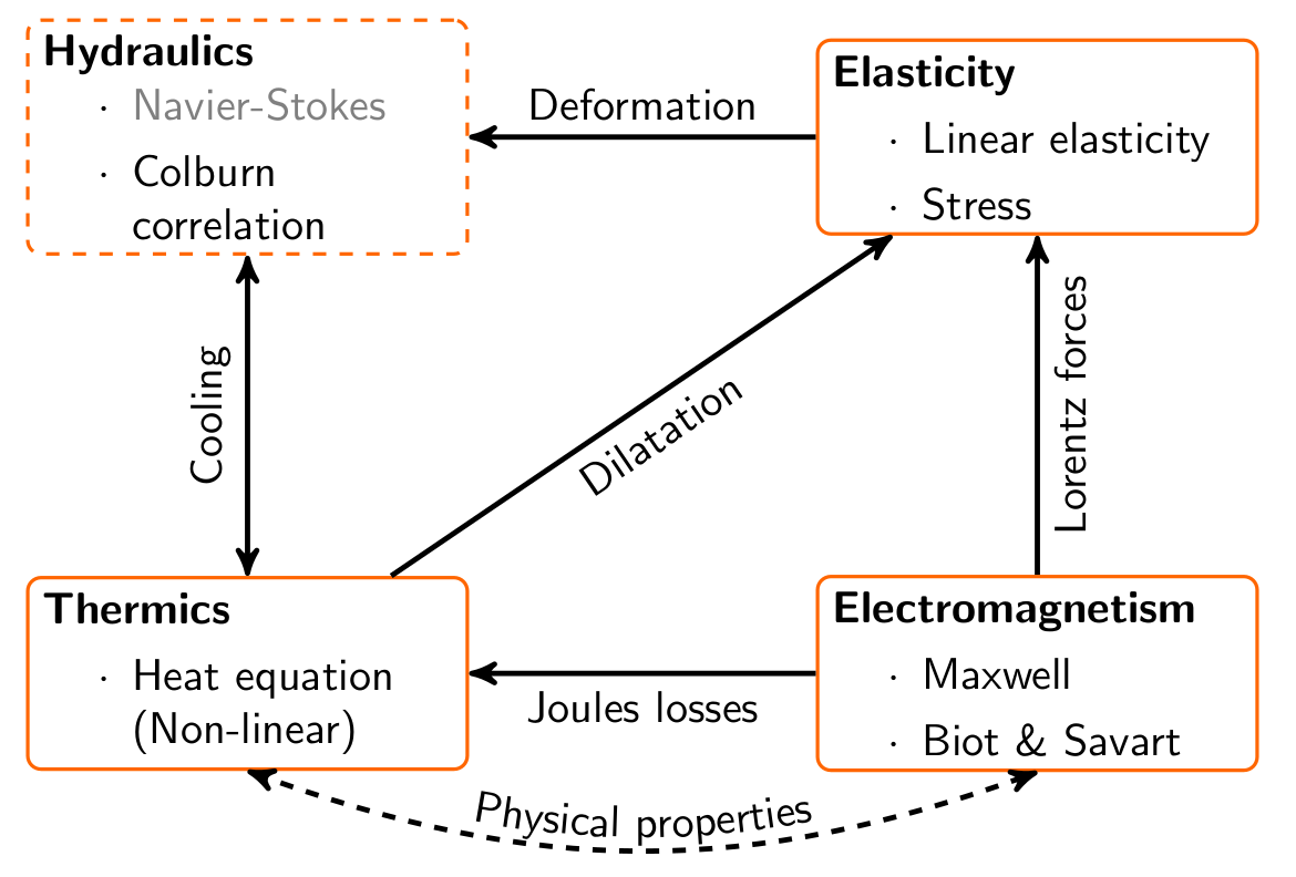
High Field Magnets modeling relies on a coupled nonlinear multiphysic model that involves:
-
electromagnetism,
-
thermics,
-
mechanics
-
and thermohydraulics for the cooling.
The nonlinearity arise from the dependencies of the physical properties of the copper alloy materials that compose the insert (ie. the so-called helices). Indeed the electrical and thermal conductivity depends on the temperature field following the Wiedemann-Frantz law: \(\frac{k(T)}{\sigma(T)\,T} = L\), where \(L\) is a material dependent constant.
The coupling of each physics is sketched in the chart bellow. Details on each physics will be given in the following sections. Finally, a specific section will be devoted to a simpler axisymetrical model used mostly for quick calculations and optimzation.
2. Conventions
In this document we will use the following convention:
-
scalar number or function will be in plain, eg \(f\)
-
vector will be in bold, \(\mathbf{f}\)
All the units used are derived from the SI system.
We will consider the usual notation for the space coordinates in \(\mathbf{R}^3\):
-
\(x,y,z\) in cartesian
-
\(r,\theta,z\) in cylindrical
4. Fields
Notation |
Quantity |
Unit |
\(T\) |
temperature |
K |
\(U\) |
electrical potential |
V |
\(\mathbf{A}\) |
magnetic potential |
\(V.s.m^{-1}\) |
\(\mathbf{B}\) |
magnetic induction |
T |
\(\mathbf{H}\) |
magnetic field |
\(A.m^{-1}\) |
5. Physical Properties
-
Thermal Properties:
Notation |
Quantity |
Unit |
\(\rho\) |
material’s density |
\(kg.m^{-3}\) |
\(C_p\) |
thermal capacity |
\(J.K^{-1}\) |
\(k\) |
thermal conductivity |
\(W.m^{-1} .K^{-1}\) |
\(\sigma\) |
electrical conductivity |
\(S.m^{-1}\) |
\(\alpha\) |
thermal resistivity coefficient |
- |
-
Magnetic Properties:
Notation |
Quantity |
Unit |
\(\mu\) |
magnetic permeability |
\(V.s.A^{-1}.m^{-1}\) |
\(\epsilon\) |
electric permittivity |
\(F.m^{-1}\) |
-
Mechanics Properties:
Notation |
Quantity |
Unit |
\(\alpha_T\) |
thermal expansion coefficient |
|
\(Y\) |
Young modulus |
\(Pa\) |
\(\nu\) |
Poisson ratio |
- |
6. Physical Quantities
Thermics:
Notation |
Quantity |
Unit |
\(h\) |
heat transfer coefficient |
\(W.m^{-2} .K^{-1}\) |
\(T_w\) |
water temperature |
\(K\) |
\(T_o\) |
reference temperature |
\(K\) |
Electromagnetism:
Notation |
Quantity |
Unit |
\(\mathbf{j}\) |
current density |
\(A.m^{-2}\) |
\(V\) |
electric potential |
\(V\) |
\(\mathbf{A}\) |
magnetic potential |
\(T.m^{-1}\) |
\(\mathbf{B}\) |
magnetic induction |
\(T\) |
\(\mathbf{H} = \mu \mathbf {B}\) |
magnetic field |
\(A.m^{-1}\) |
|
By abuse, we often refer to \(\mathbf B\) as the magnetic field. |
Mechanics:
Notation |
Quantity |
Unit |
\(P\) |
pressure |
\(Pa\) |
\({\bar{\bar{\sigma}}}\) |
stress |
\(Pa\) |
\({\bar{\bar{\epsilon}}}\) |
strain |
- |
\(\mathbf U\) |
displacement vector |
m |
7. Mathematical Functions
7.1. Usual operators
-
\(\nabla f\) : the gradient of \(f\)
-
\(\nabla \cdot \mathbf{f}\) : the divergence of \(\mathbf{f}\)
-
\(\nabla \times \mathbf{ f }\) : the curl of \(\mathbf{f}\)
7.2. Space Functions
-
\(L_{2}(\Omega)\) : \(\{f \mid \int_\Omega \|f\|^{2} < \infty\}\)
-
\(L_{2}(\Omega^d)\) : \(\{\mathbf{f} \mid \int_\Omega \|\mathbf{f}\|^{2} < \infty\}\)
-
\(H_{1}(\Omega)\) : \(\{f \in L_{2}(\Omega) \mid \nabla f \in L_{2}(\Omega^d)\}\)
-
\(H_{div}(\Omega)\) : \(\{\mathbf{f}\in L_{2} (\Omega^d) | \nabla \cdot \mathbf{f} \in L_{2}(\Omega^d)\}\)
-
\(H_{curl}(\Omega)\) : \(\{\mathbf{f}\in L_{2} (\Omega^d) | \nabla \times \mathbf{f} \in [L_{2} (\Omega^d)\}\)
By abuse we will use only \(L_{2}(\Omega)\) and not \(L_{2}(\Omega^d)\)
8. Coupled Model
8.1. Electromagnetic
The starting point of the electromagnetic model is the Maxwell equations. Using a classical approach we rewritte the equations by introducing the gauged magnetic and electric potentials, namely \(\mathbf{A}\) and \(V\). This leads to the following equation:
We add the conservation of current:
|
We use the classical Coulomb gauge to properly define the magnetic potential (ie \(\nabla \cdot \mathbf{A}=0\)). Moreover we have assume that no material exhibits an aimantation nor a polarization. |
8.1.1. QuasiStatic Maxwell (QMS)
In our case, we will neglect the second order time derivative. The final system of EDP to be solved is:
8.1.2. Magnetostatic
The steady state regime will be given by:
The boundary conditions …
Biot-Savart law
In the case of non magnetic materials (ie \(\mu=\mu_0\)), we can easily derive a solution using the Biot Savart law:
where \(G(\mathbf{X},Y)\) stands for the Green function and \(\mathbf{j} = - \sigma \nabla V\).
|
From a mathematical point of view we can refer to this solution as the fundamental solution for the laplace equation: \(- \nabla^2 \mathbf{A} = \mu_0 \mathbf{j}\). |
8.2. ThermoElectric
The temperature field \(T\) is given by the classical heat equation with the Joule losses as the source term withing \(\Omega\):
The boundary conditions associated are mainly of 3 types:
-
Homogeneous Neumann for …: \(-k \frac{\partial T}{\partial \mathbf{n}} = 0\)
-
Robin for cooled surfaces: \(-k \frac{\partial T}{\partial \mathbf{n}} = h (T-T_w)\)
-
Radiation conditons: \(-k \frac{\partial T}{\partial \mathbf{n}} = \epsilon_T T^4\)
In the current version radiation conditions are not implemented.
8.3. Elasticity
To model the mechanical behaviour of our magnets submitted to the action of Lorentz forces \(\mathbf{j} \times \mathbf{b}\), thermal expansion and to the pressure of the water flow used for the cooling, we use the classical formulation:
In testbooks the latest equation is referred as the Hooke law which represents the constitutive equation for linear material. This equation may be also expressed by:
To account for the thermal expansion of the material we add to the stress tensor \({\bar{\bar{\sigma}}}\):
with \({\bar{\bar{I}}}\) the identity tensor, and \(T_0\) is a reference temperature.
8.4. ThermoHydraulics
Cooling the magnet is mandatory to evacuate Joules losses and to keep magnet temperature bellow some heuristic limit as some copper alloys can have poor mechanical behavior at high temperature. The cooling is ensured by a forced water flow with a volumic flow rate \(Q\) up to 150 l/s.
The total heat elevation in the water \(\Delta T_w\) may be easily estimated from the electrical power \(P_e\) dissipated by the magnet using :
To model the heat exchange coefficient \(h\) we use standard thermohydraulic correlation:
with \(Re\) the Reynolds number, \(Pr\) the Prandlt number and \(D_h\) the hydraulic diameter. These quantities are defined by cooling channels:
Note that \(\mu\) stands here for the viscosity of water.
The flow velocity \(u\) per cooling channel is defined by:
where \(\Delta P\) is the pressure drop applied to force the flow (typically 25 bar), \(P_{in}\) and \(P_{out}\) are additionnal hydraulic pressure drop at the input and output of the magnet.
In practice, an alternative correlation named after B. Montgomery, who has been a pionnering engineer in the field of Magnet design, is commonly used: