MagnetTools user manual
Welcome to MagnetTools manual documentation!
MagnetTools is a in-house software for solenoidal magnets that provides tools to compute:
-
Analytically Magnetic Field,
-
Mutual and Self Inductances,
-
Axial and Radial Forces,
and to analyze some Transient Analysis.
MagnetTools also contains:
-
Optimization procedure to define the PolyHelices insert geometry,
-
Creation of Files for CAD and CAM of Helices.
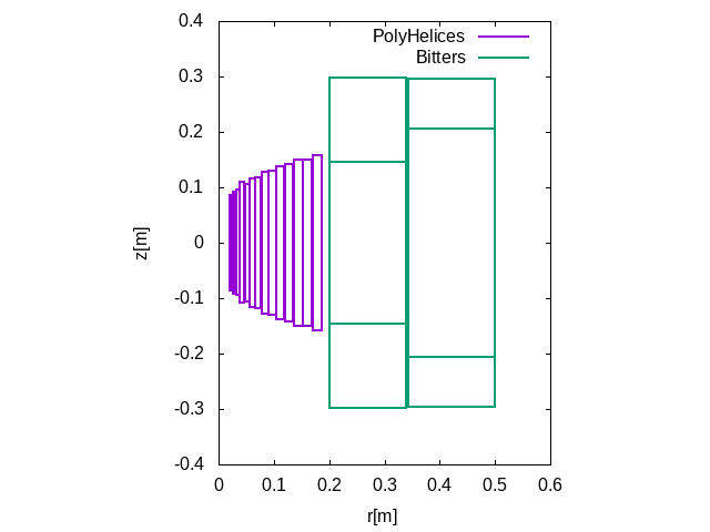
In MagnetTools, magnets are defined as a set of:
-
PolyHelices,
-
Bitter Magnets,
-
and eventually Supraconductor Magnets.
All magnets are torus of rectangular cross sections.
Quick Starts
1. Getting MagnetTools
Using MagnetTools inside container, either Docker or Singularity based, is the recommended and fastest way. If your system support singularity containers we recommend to use them instead of Docker ones.
1.1. from sregistry
MagnetTools are included in HiFiMagnet singularity image. To get HiFiMagnet singularity image see this section
1.2. from dockerhub
MagnetTools are included in HiFiMagnet docker image. To get HiFiMagnet docker image see section
1.3. from Lncmi Debian repository
On Debian/Ubuntu system you can install MagnetTools from the local Lncmi packages repository. To do so:
-
you need to have access to the Lncmi repository
-
add a
lncmi.lstinto your/etc/apt/sources.list.ddirectory:
lncmi.lst for Debian Testing distributiondeb http://euler/~trophime/debian/ testing main
deb-src http://euler/~trophime/debian/ testing mainThen run:
sudo apt update
sudo apt install hifimagnet|
Supported Debian/Ubuntu distributions:
On Windows 10 Pro you can also install HiFiMagnet without much effort. Just enable WSL feature and download Debian Stretch or Ubuntu Xenial (aka 16.04 LST) from Microsoft App Store. Then apply the same procedure as above to install the package. |
2. Using MagnetTools
2.1. Data Structure
The magnets description is given in .d file.
The .d file is structured as follows:
2.1.1. A header section:
#Power[MW]	Current[A]	Safety Ratio[]	T_ref[°C]	SymetryFlag
12.5	        31000	        0.8	        20		Sym, (1)
#Helices	N_Elem
14		56, (2)
#N   R1[m]      R2[m]      HalfL[m]    Rho[Ohm.m] Alpha[1/K] E_Max[Pa] K[W/(m.K)]   h[W/(m^2.K)] <T_W>[°C] T_Max[°C], (3)
4    1.930e-02	2.420e-02  7.7050e-02  1.992e-08  0.00e+00   3.600e+08 3.800000e+02 8.500000e+04 3.000e+01 1.00e+02
...
4    1.703e-01	1.860e-01  1.6415e-01  2.087e-08  0.00e+00   3.740e+08 3.800000e+02 8.500000e+04 3.000e+01 1.00e+02
0., (4)
#External_Magnets, (5)
0| 1 | Main parameters
|
| 2 | Main polyhelices insert characteristics:
|
| 3 | Description of each helix:
|
| 4 | flag to indicate the end of the polyhelices insert definition |
| 5 | Definitions of external magnets, if any |
2.1.2. External Magnets section
#External_Magnets (1)
6
#Type	R1[m]	R2[m] 	Z1[m]	  Z2[m]	    J(R1)[A/m2]	Rho[Ohm.m]	      Nturn (2)
1	0.2	0.34	-0.29899  -0.14685  44512000	1.7241379310345e-08   23
1	0.2	0.34	-0.14685   0.14685  86222000	1.7241379310345e-08   86
1	0.2	0.34	 0.14685   0.29899  44512000	1.7241379310345e-08   23
...| 1 | Number of external magnets, providing the background field |
| 2 | Definition of external magnet:
|
2.1.3. Resume section:
#Bz(0)[tesla]	Power[MW]	Bz_total(0)[tesla] (1)
2.754479e+01	1.250000e+01	2.754479e+01

  #Helice	B0_H[tesla]	Sum_B0[tesla]	Power_H[MW]	Sum_Power[MW] (2)
  1	       1.836561e+00	1.836561e+00	1.965246e-01	1.965246e-01
  ...
14 1.499948e+00 2.754479e+01 1.434240e+00 1.250000e+01| 1 | Main characteristics:
|
| 2 | Contribution to the self magnetic field and power per helix |
2.1.4. Detailed Helix section
  #Helix	<T>[°C]		N_Turn		IACS[%] (1)
  1	9.493052e+01	7.547479e+00	8.654981e+01
  #Elem	J[10^8 A/m2]	Tlim[°C]	Tmax[°C]	<T>[°C]		Elim[MPa]	Emax[MPa]	Pitch[m]	Nturns (2)
  1	3.477121e+00	1.000000e+02	1.000000e+02	9.493052e+01	3.600000e+02	1.803207e+02	2.041741e-02	1.886870e+00
  2	3.477121e+00	1.000000e+02	1.000000e+02	9.493052e+01	3.600000e+02	1.854755e+02	2.041741e-02	1.886870e+00
  3	3.477121e+00	1.000000e+02	1.000000e+02	9.493052e+01	3.600000e+02	1.854755e+02	2.041741e-02	1.886870e+00
  4	3.477121e+00	1.000000e+02	1.000000e+02	9.493052e+01	3.600000e+02	1.803207e+02	2.041741e-02	1.886870e+00

  ....

  #Helix	<T>[°C]		N_Turn		IACS[%]
  14	6.639741e+01	1.766565e+01	8.258438e+01
  #Elem	J[10^8 A/m2]	Tlim[°C]	Tmax[°C]	<T>[°C]		Elim[MPa]	Emax[MPa]	Pitch[m]	Nturns
  1	8.490501e-01	1.000000e+02	5.387475e+01	5.014907e+01	3.740000e+02	-4.681979e-02	2.431188e-02	3.375921e+00
  2	1.372421e+00	1.000000e+02	9.238026e+01	8.264575e+01	3.740000e+02	-1.701580e+00	1.504057e-02	5.456906e+00
  3	1.372421e+00	1.000000e+02	9.238026e+01	8.264575e+01	3.740000e+02	-1.701580e+00	1.504057e-02	5.456906e+00
  4	8.490501e-01	1.000000e+02	5.387475e+01	5.014907e+01	3.740000e+02	-4.681983e-02	2.431188e-02	3.375921e+00

MARGE DE SECURITE CONTRAINTES= 2.000000e+01 %| 1 | Stats per Helix: mean temperature, number of turns, IACS (ratio of ), |
| 2 | Details per element:
|
2.2. Magnetic Field Maps
2.2.1. Use B_Map
B_Map enables axisymetrical calculation of the magnetic field and/or potential.
See this example.
|
The first time Using the default values is generally safe.
So before entering the input currents for each part of the magnets, just press The |
Available options are:
 --points=STRING           points on which b field is to be computed (x0,y0,z0,...)
 --points_file=STRING      file containing points on which b field is to be computed (x0,y0,z0,...)
 --innerbore=INNERBORE     mesh on which b field is to be computed
 --potential               enable magnetic potential calculation / exclude magnetic field
 -domain                   perform calculations on whole mesh
 -per_elem                 perform calculations on node (default is on node)
 --sphharm=INT             perform calculations for Spherical Harmonic Decomposition [n n]
 --even_nlon               set even number of longitude
 --interactive             activate interactive mode
 --verbose                 activate verbose mode
 --magnet=INT              switch to magnet type (0: Bitter, 1: Unif, 2: ThinSolenoid, 3: PassiveShims)
 --mm                      force switch to mm as default units
 --r=DOUBLE                specify radius [default is 1 m]
 --restart_from=INT        restating computation of b field from node ID
 --save                    save results in file (default is off)
 --display                 display Helices data (default is off)
 --gnuplot                 Generate Helices Geometry data for Gnuplot (default is off)
 --ensight                 Generate Helices Geometry data for ensight (default is off)
 --ascii                   ascii write mode for ensight
 --num_integ=INT           specify num_integ size (default 100)
 --num_eval=INT            specify num_eval size (default 100)
 --gsl-error-handler       deactivate gsl error handler (default is on)
 --omp_off                 turn off openm
2.2.2. Use Levitation
Levitation computes Bz and its derivatives on Z-Axis using AD technics.
Available options are:
 --input=STRING                load input filename
 --order=INT                   specify order to consider (default is 6)
 --verbose                     activate verbose mode
 --no_ensight                  disable output for ensight
 --G0=DOUBLE                   specify G0 value to reach (default is 500)
 --residual_gravity=DOUBLE     specify residual gravity targetted in
                               percent (default is 1%)
 --check                       activate check mode (default is off)
 --find                        find levitation point (default is off)
 --save                        save results in file (default is off)
 --matlab                      save results in matlab/octave format
                               (default is off)
 --gsl-error-handler           deactivate gsl error handler (default is on)
 --interactive                 activate interactive mode
 --spec_vol=STRING             define spec vol (r, z) in m
 --sym                         activate sym mode
 --num_integ=INT               specify num_integ size (default 100)
 --num_eval=INT                specify num_eval size (default 100)
 --ascii                       ascii write mode for ensight
 --omp_off                     turn off openm
2.3. Self and Mutual Inductances
Inductances enables calculation of self and mutual inductances.
Available options are:
 --output=STRING        set output filename
 --print-detail         activate detailled printing mode
 --num-int              activate numerical integration
 --log                  activate logging mode
 --verbose              activate verbose mode
 --currents=STRING      total currents
 --tolerance=STRING     z tolerances
 --ntol=STRING          ntol tolerances case
 --grid=STRING          ni nj grid size
2.4. Force Field Maps
2.4.2. Radial Forces and Torques
Forces enables the calculations of forces and torques in case of radial misalignement of magnet axis. Available options are
 --output=STRING          set output filename
 --input=STRING           load input filename
 --save=STRING            save input data to filename
 --rotation=STRING        OxOz angle between z-axis (in deg)
 --translation=STRING     translations between Magnetic Center and Origin
 --grid=STRING            nr nz ntheta grid size
 --verbose                activate verbose mode
2.4.3. Connection with CSM software (eg Samcef, Ansys )
F_Map
 -f, --input_format=INPUT_FORMAT     input mesh format (eg, .dat)
 --density=DOUBLE                specify density (default is nan)
 --verbose                       activate verbose mode
 --mm                            force switch to mm as default units
 --ascii                         ascii write mode for ensight
 --samcef                        Generate Samcef Forces data for Samcef
                                 (default is off)
 --ansys                         Generate Ansys Forces data for Ansys
                                 (default is off)
 --num_integ=INT                 specify num_integ size (default 100)
 --num_eval=INT                  specify num_eval size (default 100)
 --gsl-error-handler             deactivate gsl error handler (default is
2.5. Transient Analysis
-
power failure
-
matrix exponential
-
powerfailure enables simulations of transients (ie. power failure) using expokit
-
implicit/explicit euler
transient_ida enables simulations of transients (ie. power failure) using Sundials IDA lib. Available options are
 --init=STRING            set init_current filename
 --output=STRING          set output filename
 --input=STRING           load input filename
 --save=STRING            save input data to filename
 --solver=INT             activate solver (0: dense, 1:gmres, 2:tfqmr)
 --params=STRING          load solver params from file
 --verbose                activate verbose mode
 --quench                 activate quench mode (add quench resistance to supra
 --aubert                 activate aubert init. current calculation mode
 --screen=INT             add screen definition
 --burnout=STRING         index of the bitter external magnet with a short-circuit (i j)
 --shorted_in_series      bitter external magnet(s) with a short-circuit are in series (0: false by default)
 --tolerance=DOUBLE       specify Optimaly tolerance (default is 1.0e-4)
 --grid_size=STRING       set grid size of B calculation (r0 r1 z0 z1)
 --grid_dim=STRING        set grid dim of B calculation (n_r n_z)
 --ascii                  ascii write mode for ensight
 --induct_file=STRING     save/load inductances from file
 --fz_file=STRING         save/load forces from file
 --num_integ=INT          specify num_integ size (default 100)
 --num_eval=INT           specify num_eval size (default 100)
 --no_ensight             disable output for ensight
--omp_off turn off openm-
critical scenario: bitter burnout
2.6. Optimization
The goal of the Axisymetric optimization is to provide an maximum magnetic field at the center of the insert under constraints:
-
total electric power
-
maximal allowed temperature per helix
-
maximal allowed stress per helix
for a given insert geometry.
The unknowns may either be:
-
the current density distribution per helix:
OptHelix, -
the maximum temperature distribution per helix:
OptAubert
OptAubert HL-31.dat|
Each helix is splitted in a given number of sections \(S_i\) along \(z\) axis.
The result of the optimization is the vector stem[{j_i}] (aka the current density \(j_i\) value on the inner radius of
all sections \(S_i\)) for The stress in each section is approximated by the Hoop stress, namely \(r j_{\theta}(r) \cdot b_z(r)\) for \(r=r_i\) with \(r_i\) the inner radius of section \(S_i\). |
|
Both codes relies on SQP programming with |
The input file corresponds to the header section of the .d magnet description file.
The output is a .d file.
To build the actual 3D geometry, that shall reflect, this axisymetrical current density distribution, we use the following assumption:
-
the nominal current is \(I_o\),
-
each element \(S_i\) will be represented by an helix with a pitch \(p\) and a number of turn \(n\) such that the helix carries the same current as the element:
The optimization result are then used to define the helical cut thet would be machined in each copper alloy tubes:
-
CAD data may be obtained for Catia and/or Salome using:
opt2cad HL-31.d , (1)
addshape ... , (2)
opt2yml HL-31.d , (3)| 1 | opt2cad generates files for CAD/CAM Helices |
| 2 | addshape generates files for CAD/CAM Helices with "bumps" on the helical cut shape path; this is optional. |
| 3 | opt2yml generates configuration files for building Helices with HiFiMagnet Salome plugin. |
| To create the actual 3D CAD model of an helix (abusively: tube in which an helical cut has been machined by EDM technic), we still need some more information… |
2.6.1. Use OptAubert
optaubert HL-31.datAvailable options to control the optimization are:
--majorprint=INT                specify nag major print level (default is 10)
--minorprint=INT                specify nag major print level (default is 0)
--major_iteration_limit=INT     specify nag major iterations_limit (default is controlled by nag)
--minor_iteration_limit=INT     specify nag minor iterations_limit (default is controlled by nag)
--tolerance=DOUBLE              specify Optimaly tolerance (default is 1.0e-15)
--function_precision=DOUBLE     specify Function precision (default is 4.38e-15)
--feasibility=DOUBLE            specify nonlinear feasibility tolerance (default is 1.0e-15)
--check                         activate nag checks
--random                        initiliaze with random numbers
--init=STRING                   initialize solution from
--verbose                       activate verbose mode
--log                           activate nag logging mode
--recursive                     activate recursive mode
Other options are:
--gmsh                          activate gmsh output
--num_integ=INT                 specify num_integ size (default 100)
--num_eval=INT                  specify num_eval size (default 100)
--gsl-error-handler             deactivate gsl error handler (default is on)
2.6.2. Use OptHelix
opthelix --stress --temp [--cooling] [--geom] HL-31.datAvailable options are:
--majorprint=INT                specify nag major print level (default is 10)
--minorprint=INT                specify nag major print level (default is 0)
--major_iteration_limit=INT     specify nag major iterations_limit (default is controlled by nag)
--minor_iteration_limit=INT     specify nag minor iterations_limit (default is controlled by nag)
--tolerance=DOUBLE              specify Optimaly tolerance (default is 1.0e-15)
--feasibility=DOUBLE            specify nonlinear feasibility tolerance (default is 1.0e-15)
--geom                          activate geometry optimization
--check                         activate nag checks
--temp                          activate temperature constraints
--stress                        activate stress constraints
--random                        initiliaze with random numbers
--gmsh                          activate gmsh output
--init=STRING                   initialize solution from
--verbose                       activate verbose mode
--log                           activate nag logging mode
--recursive                     activate recursive mode
--cooling                       activate cooling modeling
--num_integ=INT                 specify num_integ size (default 100)
--num_eval=INT                  specify num_eval size (default 100)
2.6.3. Generating CAD/CAM files
To create files for CAD or CAM use opt2cad:
opt2cad [-o format] HL-31.dValid formats are:
-
LNCMI: default value, for creating file for Lncmi CAM -
CATIA: for creating files for CATIA -
SALOME: for creating files for Salome
To add shapes on some helical cuts, you may use:
add_shape --angle="60 90 120 120" --shape_angular_length=8 --shape=HL-31-995 --format=LNCMI --position="ALTERNATE" HL-31_H4In this example we had shape profile HL-31-995 at various angles on HL-31_H4 helical cut.
HL-31-995: Shape_HL-31-995.dat#Shape : HL-31-995 pour H4
#N_i
20
#X_i F_i
-3.24 0
-3.05 0.04
-2.88 0.15
-2.78 0.31
-2.74 0.5
-2.74 1.3
-2.7 1.49
-2.59 1.65
-2.43 1.76
-2.24 1.8
2.24 1.8
2.43 1.76
2.59 1.65
2.7 1.49
2.74 1.3
2.74 0.5
2.78 0.31
2.88 0.15
3.05 0.04
3.24 0This command will generate 2 files:
-
HL-31_H4_cut_with_shapes.iso: CAM file for the EDM machining, -
HL-31_H4_cut_with_shapes.xls: CAD file for CATIA (the file needs to be converted to a real Excell file with the scriptwrite_excel.py)
2.6.4. Prepare Data for HiFiMagnet Salome
opt2yml HL-31.dThis command generates .yaml cfg files for Helices.
These files are, somehow, incomplete.
Some information has to be added to be complete, eg the dimension of the tube correspond to the actual helix.
|
To add shapes on some helical cuts, you may use |