Magnetic Field Gradient Map (Axisymetric geom)
In this example, we will compute the "ideal" magnetic field and its gradient produced by a test insert described using MagnetTools format.
1. Running the case
To run this example on MSO4SC portal see this section.
1.1. Magnet Geometry
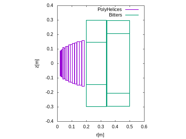
|
To get the geometry, you can use: Edit Plot the geometry with |
1.2. Magnet Field
To compute the magnetic field:
Levitation HL-31.dthen enter the data for:
-
Helix input current,
-
Bitter input current,
-
and eventually Supra outsert input current.
The result is stored in HL-31_dev.dat.
|
On first run, you will need to enter some more parameters before entering the currents and plot ranges data
if you don’t have an On MSO4SC Data Catalogue this file is already included in the dataset. |
For instance using the default current params, you get the following magnetic field \(B_z\) profile along \(Oz\) axis as long as its gradient.
There are others usefull options to carry out calculation on list of points and so on.
See here for details.
2. Data files
The data files may be retreived from Data Catalogue. See the dataset HL-31 in Lncmi collection.
The gzipped archive tarball HL-31-ana.tgz contains all the files needed.
3. Outputs
The value of Magnetic Field in cylindrical coordinates at \((r=0,z=0)\) is: \((0,37.8622880853634)\)
To view the result with gnuplot in the remote desktop, type the following command:
plot "HL-31_dev.dat" using 1:2 w l lw 3 title "B_z", \
     "HL-31_dev.dat" using 1:3 axis x1y2 w l lw 3 title "dB_z/dz"
profile on \(Oz\) axis]