Formulation

1. Differential form of Maxwell’s equations

Maxwell’s equations, are laws of physics, constituting the basic postulates of electromagnetism. They translate, in local form, several theorems that governed electromagnetism, that Maxwell gathered in integral form. These equations define relations between the electromagnetic fields and the source elements. The differential form of Maxwell’s equations is as follows:

\[\begin{align*} \nabla \times H(r,t) &=& J(r,t) + \frac{\partial D(r,t)}{\partial t} \\ \nabla \times E(r,t) &=& -\frac{\partial B(r,t)}{\partial t} \\ \nabla \cdot B(r,t) &=& 0 \\ \nabla \cdot D(r,t) &=& \rho(r,t) \\ B(r,t) &=& \mu_0[H(r,t)+M(r,t)] \\ J(r,t) &=& \sigma[E(r,t)+E_i(r,t)] \\ D(r,t) &=& \epsilon_0 E(r,t) + P(r,t) \end{align*}\]

where :

\(H(r,t)\)

the magnetic field intensity,

\(E(r,t)\)

the electric field intensity,

\(B(r,t)\)

the magnetic flux density,

\(D(r,t)\)

the electric flux density,

\(J(r,t)\)

the electric current density,

\(\rho(r,t)\)

the electric charge density,

\(M(r,t)\)

the magnetization,

\(E_i(r,t)\)

the impressed electric field,

\(P(r,t)\)

the polarization,

\(\mu_0(r,t)\)

the permeability of vaccum,

\(\sigma(r,t)\)

the conductivity,

\(\epsilon_0(r,t)\)

the permittivity of vacuum.

2. The magnetic vector and electric scalar potentials formulation

We’re interested in simplified equations:

\[\begin{align*} \nabla \times H(r,t) &=& J(r,t) + \frac{\partial D(r,t)}{\partial t} \\ \nabla \times E(r,t) &=& -\frac{\partial B(r,t)}{\partial t} \\ \nabla \cdot B(r,t) &=& 0 \\ \nabla \cdot D(r,t) &=& 0 \\ B(r,t) &=& \mu_0H(r,t) \\ D(r,t) &=& \epsilon_0 E(r,t) \\ J(r,t) &=& \sigma E(r,t) \end{align*}\]

The MQS approximation consists in neglecting the so-called displacement current, aka \(\frac{\partial D}{\partial t}\). In this context, the equations to solve are:

\[\begin{align} \nabla \times H(r,t) &=& J(r,t),\label{Ampere} \\ \nabla \times E(r,t) &=& -\frac{\partial B(r,t)}{\partial t}, \label{Faraday} \\ B(r,t) &=& \mu_0H(r,t) \\ J(r,t) &=& \sigma\,E(r,t) \end{align}\]
The first two equations are respectively the so-called Ampere and Faraday equations.

A classical way to solve these equations is to introduce a magnetic potential \(A\) and a scalar electric potential \(V\). As \(B\) is a divergence free field, we can define \(A\) as:

\[\begin{equation*} B = \nabla \times A. \end{equation*}\]

To ensure \(A\) unicity we will need to add a gauge condition. Most commonly:

\[\begin{equation*} \nabla \cdot A = 0 \end{equation*}\]

The Faraday equation may, then, be rewritten as:

\[\begin{equation*} \nabla \times (E +\frac{\partial A}{\partial t} ) = 0. \end{equation*}\]

We can define the electric scalar potential \(V\) as:

\[\begin{equation*} E +\frac{\partial A}{\partial t} = -\nabla V. \end{equation*}\]

It follows that:

\[\begin{equation*} J = \sigma ( -\nabla V -\frac{\partial A}{\partial t}). \end{equation*}\]

From this expression of the current density, we may rewrite the Ampere equation as:

\[\begin{equation} \nabla \times (\frac{1}{\mu}\,\nabla \times A) + \sigma \frac{\partial A}{\partial t} = -\sigma \, \nabla V.\quad\text{(1)}\label{nAmpere} \end{equation}\]

because :

\[\begin{equation*} B = \nabla \times A = \mu H \end{equation*}\]

so :

\[\begin{equation*} \nabla \times H = \nabla \times ( \frac{1}{\mu} \nabla \times A) \end{equation*}\]

To this equation, we add the conservation of the current density:

\[\begin{equation} \nabla \cdot (J) = \nabla \cdot (\sigma ( -\nabla V -\frac{\partial A}{\partial t})) = 0\quad\text{(2)} \end{equation}\label{nConservation}\]

Equations (1) and (2) are the equations that we will solve for the MQS model.

3. Weak formulation

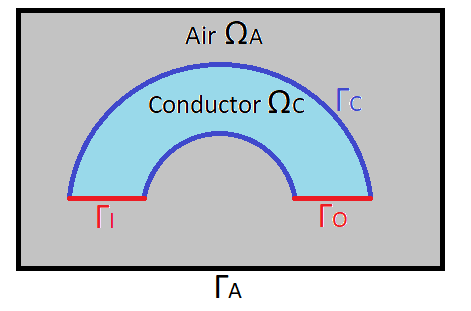
Let us note \(\Omega\) the domain, comprising the conductor \(\Omega_C\) and the air \(\Omega_A\), and let us note \(\Gamma\) the edge of this domain, comprising the edge of the air \(\Gamma_A\), the inlet \(\Gamma_I\) and the outlet \(\Gamma_O\). To simplify, let us note \(\Gamma_D\) the edges with Dirichlet boundary condition, and \(\Gamma_N\) the edges with Neumann bondary condition, such that \(\Gamma = \Gamma_D \cup \Gamma_N\).

geometry

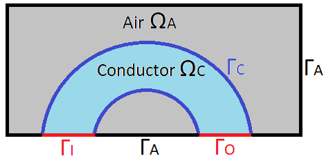
We can also have a second case where the edges \(\Gamma_I\) and \(\Gamma_O\) are on \(\Gamma_A\), where we can impose Dirichlet boundary condition.

geometry

Let’s look at the set:

\[\begin{equation} H^{curl}(\Omega) = \{v \in L^2(\Omega)| \nabla \times v \in L^2(\Omega)\} \end{equation}\]

and let define the set containing Dirichlet’s boundary condition :

\[\begin{equation} H_{A_D}^{curl}(\Omega) = \{v \in H^{curl}(\Omega)| v \times n = A_D \text{ on } \Gamma_D\} \end{equation}\]

We can now distinguish two cases. First, if the edges are not curved, we have the following case, where \(A_D = 0\) :

Let us consider the equation (1) : By making the scalar product with \(\phi \in H_{A_D}^{curl}(\Omega)\) and by integrating on \(\Omega\) we get :

\[\begin{equation} \int_{\Omega} \phi \cdot (\nabla \times (\frac{1}{\mu}\,\nabla \times A) + \sigma \frac{\partial A}{\partial t}) = \int_{\Omega_C} \phi \cdot (-\sigma \, \nabla V) \end{equation}\]

Using the relationship:

\[\nabla \cdot (u \times v) = v \cdot (\nabla \times u) - u \cdot (\nabla \times v)\]

we deduce that:

\[\begin{equation} \int_{\Omega} \frac{1}{\mu} \, (\nabla \times \phi) \cdot (\nabla \times A) + \int_{\Omega} \frac{1}{\mu} \nabla \cdot (\phi \times (\nabla \times A)) = - \int_{\Omega_C} \sigma \phi \cdot (\nabla V + \frac{\partial A}{\partial t}) \end{equation}\]

Using the divergence theorem we get:

\[\begin{equation} \int_{\Omega} \frac{1}{\mu} \, (\nabla \times \phi) \cdot (\nabla \times A) + \int_{\Gamma_D} \frac{1}{\mu} (\phi \times (\nabla \times A))\cdot n + \int_{\Gamma_N} \frac{1}{\mu} (\phi \times (\nabla \times A))\cdot n = - \int_{\Omega_C} \sigma \phi \cdot (\nabla V + \frac{\partial A}{\partial t}) \end{equation}\]

By performing a circular permutation on \(\Gamma_N\) and \(\Gamma_D\) we have :

\[\begin{equation} \int_{\Omega} \frac{1}{\mu} \, (\nabla \times \phi) \cdot (\nabla \times A) - \int_{\Gamma_D} \frac{1}{\mu} (\phi \times n) \cdot (\nabla \times A) + \int_{\Gamma_N} \frac{1}{\mu} ((\nabla \times A) \times n ) \cdot \phi = - \int_{\Omega_C} \sigma \phi \cdot (\nabla V + \frac{\partial A}{\partial t}) \end{equation}\]

On \(\Gamma_N\) we impose homogeneous Neumann boundary conditions \(B \times n = 0\) since \(B = \nabla \times A\). This condition typically apply for physical symetry on some bounday (cf 1/8 of a torus example). So \((\nabla \times A) \times n = 0\) on \(\Gamma_N\). On \(\Gamma_D\) we impose Dirichlet boundary condition \( \phi \times n = A_D\), where \(A_D\) is known.

In the case where edges are not curved, we have \( \phi \times n = A_D = 0\). So we finally get the weak formulation:

\[\begin{equation} \int_{\Omega} \frac{1}{\mu} \, (\nabla \times \phi) \cdot (\nabla \times A) = - \int_{\Omega_C} \sigma \phi \cdot (\nabla V + \frac{\partial A}{\partial t}) \end{equation}\]

In the second case, were we have curved edges, we concider that \( \phi \times n = A_D\), where \(A_D\) is known.

So we have :

\[\begin{equation} \int_{\Omega} \frac{1}{\mu} \, (\nabla \times \phi) \cdot (\nabla \times A) - \int_{\Gamma_D} \frac{1}{\mu} A_D \cdot (\nabla \times A) = - \int_{\Omega_C} \sigma \phi \cdot (\nabla V + \frac{\partial A}{\partial t}) \end{equation}\]

The border of \(\Omega_C\) is considered to be splitted into \(\Gamma_I\), \(\Gamma_O\) respectively the input and output of current and the rest will be noted \(\Gamma_C\). On \(\Gamma_I\) and \(\Gamma_O\) we consider Dirichlet Boundary condition for the electrical potential. Thus we will take \(\psi \in H^1(\Omega_C)\).

Let’s consider the equation (2) : By making the scalar product with \(\psi\) and integrating over \(\Omega_C\) we get :

\[\begin{equation} \int_{\Omega_C} \psi \cdot \nabla \cdot (\sigma ( -\nabla V -\frac{\partial A}{\partial t})) = 0 \end{equation}\]

Using the relationship:

\[\nabla \cdot (u \cdot v) = v \cdot \nabla u + u \nabla \cdot v\]

we get :

\[\begin{equation} \int_{\Omega_C} \nabla \cdot (\sigma \psi \cdot ( -\nabla V -\frac{\partial A}{\partial t})) - \int_{\Omega_C} \sigma ( -\nabla V -\frac{\partial A}{\partial t}) \cdot \nabla \psi = 0 \end{equation}\]

By using the formula of divergence we get:

\[\begin{equation} \int_{\Gamma_C} \sigma \psi \cdot ( -\nabla V -\frac{\partial A}{\partial t}) \cdot n - \int_{\Omega_C} \sigma ( -\nabla V -\frac{\partial A}{\partial t}) \cdot \nabla \psi = 0 \end{equation}\]

Or we know that \(j \cdot n = 0\) on \(\Gamma_C\) due to the current density conservation law. Or \(j = \sigma E = \sigma(\nabla V + \frac{\partial A}{\partial t})\) so we get finally :

\[\begin{equation} - \int_{\Omega_C} \sigma ( -\nabla V -\frac{\partial A}{\partial t}) \cdot \nabla \psi = 0 \end{equation}\]