Implementation

To implement the two discretized equations obtained in the discretization paragraph, we will first program the resolution of the first equation and then of the second one. Finally, we will implement the two equations together, and solve the system.

1. First equation

Remember that for the first equation we have :

\[\begin{equation} \int_{\Omega} \frac{\Delta t}{\mu} \, (\nabla \times \phi) \cdot (\nabla \times A^n) - \int_{\Gamma_D} \frac{1}{\mu} A_D \cdot (\nabla \times A^n) + \int_{\Omega_C} \sigma \phi \cdot (A^n + \Delta t \nabla V) = \int_{\Omega_C} \sigma \phi \cdot A^{n-1} \end{equation}\]

To solve the first equation only, we will assume that V is known. By slightly transforming the first equation, we obtain :

\[\begin{equation} \int_{\Omega} \frac{\Delta t}{\mu} \, (\nabla \times \phi) \cdot (\nabla \times A^n) - \int_{\Gamma_D} \frac{1}{\mu} A_D \cdot (\nabla \times A^n) + \int_{\Omega_C} \sigma \phi \cdot A^n = \int_{\Omega_C} \sigma \phi \cdot (A^{n-1} - \Delta t \nabla V) \end{equation}\]

We will now implement this equation under feelpp. First, we define the \(\Omega\), the domain, as well as the \(\Omega_C\), the sub-domain of the conductor.

auto mesh = loadMesh(_mesh = new Mesh<Simplex<3>>);
auto cond_mesh = createSubmesh(mesh, markedelements(mesh, "Omega_C"));

Remember that \(A \in H_{A_D}^{curl}\), but here, to simplify, we will consider that \(A \in H^{1}\), so we have to take a correct function space for \(A^n\) :

auto Ah = Pchv<1>(mesh);

We now define all of our elements :

auto A = Ah->element(A0);
auto phi = Ah->element();
auto Aexact = Ah->element();

Where \(Aexact\) is the exact solution of a given problem, and where A is initialized with \(A0\).

Then we create the first and second member of the weak formulation, the exporter and the time variable.

auto l1 = form1(_test = Ah);
auto a1 = form2(_trial = Ah, _test = Ah);
double t = 0;
auto e = exporter(_mesh = mesh);

We define result at time 0, the \(H^1\) and \(L^2\) errors.

Vexact_g.setParameterValues({{"t", t}});
Vexact = project(_space = Vh, _expr = Vexact_g);

gradV.setParameterValues({{"t", t}});
e->step(t)->add("V", V0);
e->step(t)->add("Vexact", Vexact);
e->save();

double L2Vexact = normL2(_range = elements(mesh), _expr = Vexact_g);
double H1error = 0;
double L2error = 0;

We then begin the time loop, were we write the first and second member at time t :

Aexact_g.setParameterValues({{"t", t}});
Aexact = project(_space = Ah, _expr = Aexact_g);
gradV.setParameterValues({{"t", t}});
gO.setParameterValues({{"t", t}});
gI.setParameterValues({{"t", t}});
Ad.setParameterValues({{"t", t}});

l1.zero();
a1.zero();
l1 = integrate(_range = elements(cond_mesh),
                _expr = sigma * inner(id(phi), idv(A) - dt * gradV));
a1 = integrate(_range = elements(mesh),
                _expr = (dt / mu) * inner(curl(phi), curlt(A)));
a1 += integrate(_range = elements(cond_mesh),
                _expr = sigma * inner(id(phi), idt(A)));
a1 += on(_range = markedfaces(mesh, "Gamma_I"), _rhs = l1, _element = phi,
         _expr = gI);
a1 += on(_range = markedfaces(mesh, "Gamma_O"), _rhs = l1, _element = phi,
         _expr = gO);
a1 += on(_range = markedfaces(mesh, "Gamma_C"), _rhs = l1, _element = phi,
         _expr = Ad);

Finally, we finish by solving the equation at time t, exporting the result, and error calculations.

a1.solve(_rhs = l1, _solution = A);

e->step(t)->add("A", A);
e->step(t)->add("Aexact", Aexact_g);
e->save();

L2Aexact = normL2(_range = elements(mesh), _expr = Aexact_g);
L2error = normL2(elements(mesh), (idv(A) - idv(Aexact)));
H1error = normH1(elements(mesh), _expr = (idv(A) - idv(Aexact)), _grad_expr = (gradv(A) - gradv(Aexact)));

And we start the loop again, which end when \(t \geq tmax\).

Complete code is available in the code section.

Now, we will test this program using the function \(V = (-xz,0,-\frac{t}{\sigma})\) with \(\sigma = 58000\) and \(\mu = 1\). Note that the exact solution \(A\) for this \(V\) is \(A = (xzt,0,0)\).

We will also take the time \(t \in [0,1]\), with a step time \(dt=0.025\).

We’ll run the simulation on a bar, representing the conductor.

geometry

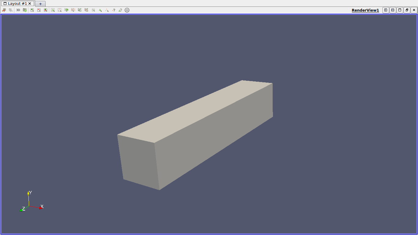
This is the config file of the simulation :

directory=hifimagnet/mqs/test1

[gmsh]
hsize=0.1
filename=$cfgdir/test1.geo

[functions]
a={0,0,0}
i={x*z*t,0,0}:x:y:z:t
o={x*z*t,0,0}:x:y:z:t
d={x*z*t,0,0}:x:y:z:t
v={-x*z,0,-t/58000}:x:y:z:t
m=1
s=58000
e={x*z*t,0,0}:x:y:z:t

[ts]
time-step = 0.025
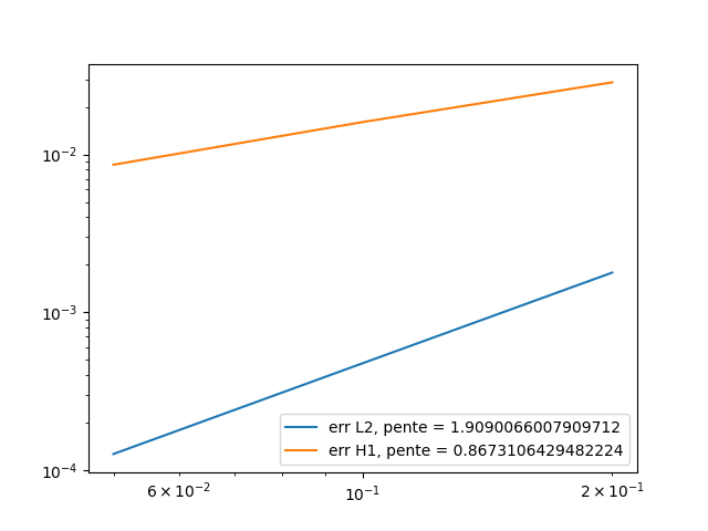
time-final = 1

Below are the errors we get at different times, with the associated graph in log scale.

\(t=0.1\):

h	0.2	0.1	O.05
\(L^2\) error	0.000198386	5.29439e-05	1.40537e-05
\(L^2\) relative error	0.000532326	0.000142063	3.77101e-05
\(H^1\) error	0.00318232	0.00178333	0.000950294

geometry

\(t=0.5\):

h	0.2	0.1	O.05
\(L^2\) error	0.000992004	0.000264656	7.02804e-05
\(L^2\) relative error	0.000532365	0.000142029	3.77164e-05
\(H^1\) error	0.0159153	0.00891686	0.00476399

geometry

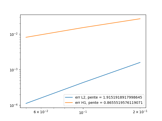
\(t=0.9\):

h	0.2	0.1	O.05
\(L^2\) error	0.00178574	0.000476291	0.000126614
\(L^2\) relative error	0.000532405	0.000142003	3.77491e-05
\(H^1\) error	0.0286545	0.0160523	0.00861033

geometry

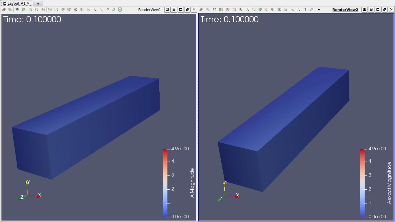
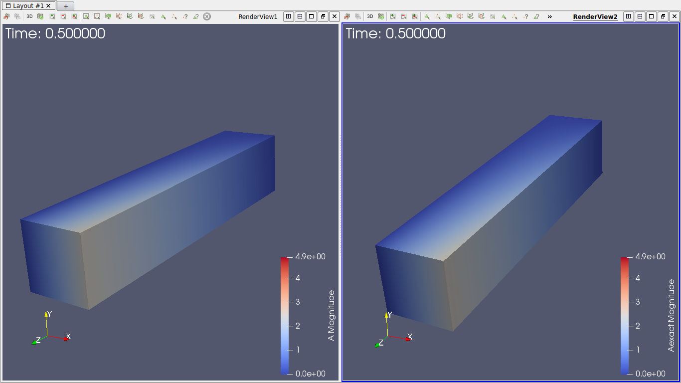
Here is a comparison under paraview between the exact solution and the calculated solution, at different time :

geometry

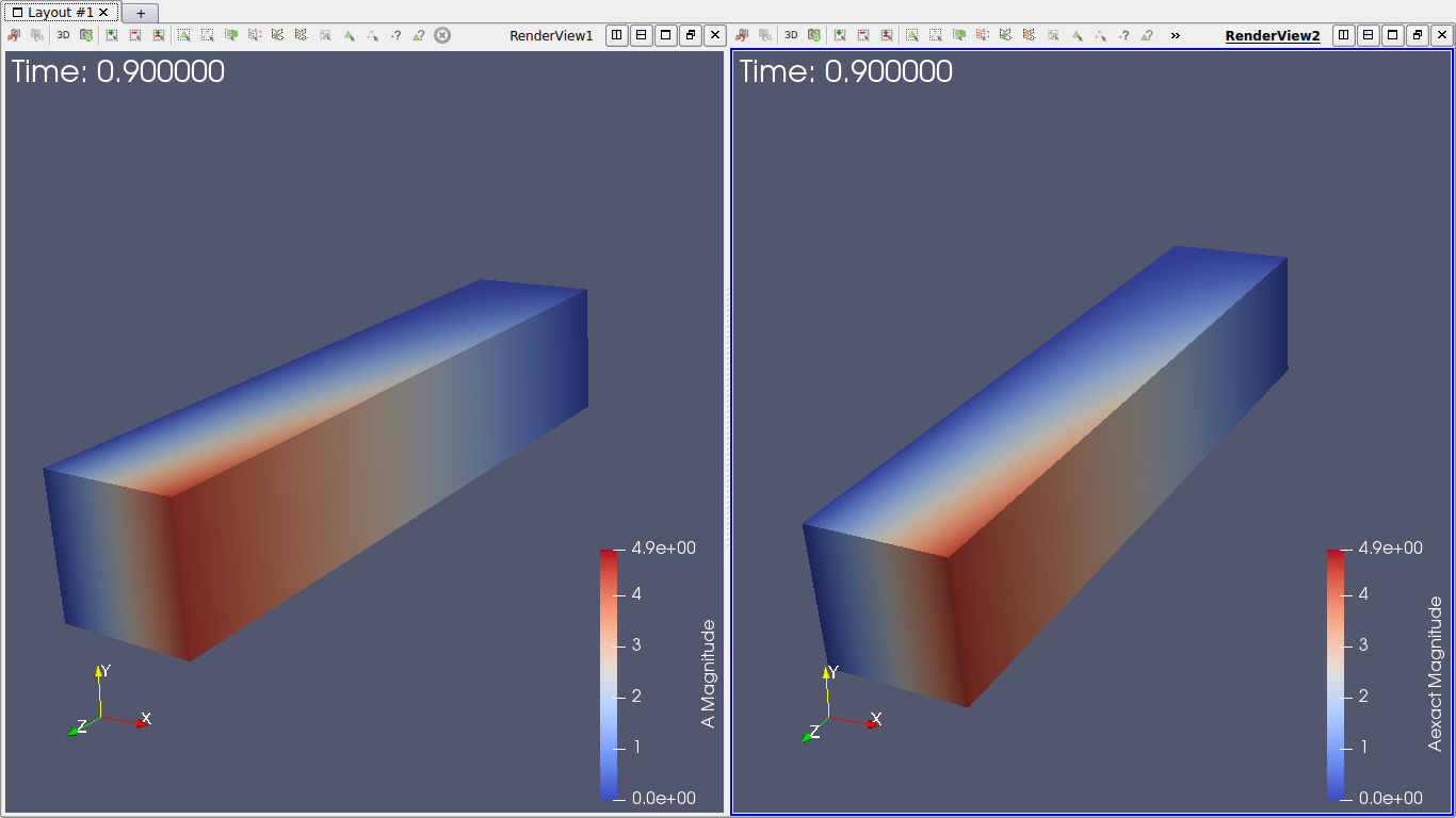
We conclude that at every time, the \(L^2\) error slope is close to 2, which is what we expect to have, and the \(H^1\) error slope is also close to 1. The difference can be explain by the fact we took only 3 different hsize, and the result could be better with lower hsize (but the running time can become very long).

2. Second equation

Our second equation is :

\[\begin{equation} \int_{\Omega_C} \sigma (A^n + \Delta t\nabla V) \cdot \nabla \psi = \int_{\Omega_C} \sigma A^{n-1} \cdot \nabla \psi \end{equation}\]

To solve the second equation only, we will assume that \(\frac{\partial A}{\partial t}\) is known. By slightly transforming this equation, we obtain :

\[\begin{equation} \int_{\Omega_C} \sigma \nabla V \cdot \nabla \psi = - \int_{\Omega_C} \frac{\partial A}{\partial t} \cdot \nabla \psi \end{equation}\]

The code is almost the same as before, with a few modifications :

First, we change our function space :

auto Vh = Pch<1>( cond_mesh );

and we define our elements :

auto V = Vh->element(V0);
auto psi = Vh->element();
auto Vexact = Vh->element();

Then we define our two forms :

auto a2 = form2( _trial=Vh, _test=Vh);
auto l2 = form1( _test=Vh );
auto e = exporter( _mesh=mesh );

The last change is inside the loop, were we define the second equation :

l2 = integrate(_range=elements(cond_mesh),_expr = sigma * inner( -dA, trans(grad(psi)) ));

a2 = integrate(_range=elements(cond_mesh),_expr = sigma * inner(gradt(V), grad(psi) ));

a2 += on(_range=markedfaces(cond_mesh,"Gamma_I"), _rhs=l2, _element=psi, _expr= gI );
a2 += on(_range=markedfaces(cond_mesh,"Gamma_O"), _rhs=l2, _element=psi, _expr= gO );
a2 += on(_range=markedfaces(cond_mesh,"Gamma_C"), _rhs=l2, _element=psi, _expr= Ad );

Then we solve, and we compute the errors.

Complete code is available in the code section.

Now we will test this program with two different set of function : First will be with the function \(A = (-t,0,0)\), so \(\frac{\partial A}{\partial t} = (-1,0,0)\). Note that the exact solution is \(V = zt\).

We will run the simulation on the same geometry as before, with same time and step time.

This are the errors we get with hsize = 0.1 :

0.1

0.5

O.9

\(L^2\) error

1.40624e-15

3.01653e-15

7.75481e-15

\(L^2\) relative error

2.17853e-15

9.34637e-16

1.33486e-15

\(H^1\) error

4.47471e-15

2.05823e-14

3.85823e-14

The error is 0 at epsilon machine, which is what is expected because the function is linear in space.

This is the config file for this simulation :

directory=hifimagnet/mqs/test2

[gmsh]
hsize=0.1
filename=$cfgdir/test2.geo

[functions]
v=0
a={-t,0,0}:x:y:z:t
i=z*t:x:y:z:t
o=z*t:x:y:z:t
d=z*t:x:y:z:t
s=58000
e=z*t:x:y:z:t

[ts]
time-step = 0.025
time-final = 1

Now we will use the function \(A = (-xt,0,zt)\), so \(\frac{\partial A}{\partial t} = (-x,0,z)\). Note that the exact solution is \(V = zxt\).

We will run the simulation on the same geometry as before, with same time and step time.

Below are the errors we get at different times, with the associated graph in log scale.

\(t=0.1\):

h	0.2	0.1	O.05
\(L^2\) error	0.000318572	8.66208e-05	2.23948e-05
\(L^2\) relative error	0.00085482	0.000232428	6.00916e-05
\(H^1\) error	0.00537588	0.00303521	0.00161933

geometry

\(t=0.5\):

h	0.2	0.1	O.05
\(L^2\) error	0.00159286	0.000433104	0.000111974
\(L^2\) relative error	0.00085482	0.000232428	6.00916e-05
\(H^1\) error	0.0268794	0.0151761	0.00809665

geometry

\(t=0.9\)

h	0.2	0.1	O.05
\(L^2\) error	0.00286715	0.000779587	0.000201553
\(L^2\) relative error	0.00085482	0.000232428	6.00916e-05
\(H^1\) error	0.0483829	0.0273169	0.014574

geometry

Here is a comparison under paraview between the exact solution and the calculated solution, at different time:

geometry

This is the config file of the simulation :

directory=hifimagnet/mqs/test22

[gmsh]
hsize=0.1
filename=$cfgdir/test2.geo

[functions]
v=0
a={-x*t,0,z*t}:x:y:z:t
i=x*z*t:x:y:z:t
o=x*z*t:x:y:z:t
d=x*z*t:x:y:z:t
s=58000
e=x*z*t:x:y:z:t

[ts]
time-step = 0.025
time-final = 1

We can conclude that the \(L^2\) and \(H^1\) errors are what expected, for the same reason as first equation.

3. Coupled system

Now we take back our system :

\[\begin{equation} \int_{\Omega_C} \sigma (A^n + \Delta t\nabla V) \cdot \nabla \psi = \int_{\Omega_C} \sigma A^{n-1} \cdot \nabla \psi \end{equation}\]

Which can be rewrite :

\[\begin{equation} \int_{\Omega} \frac{\Delta t}{\mu} \, (\nabla \times \phi) \cdot (\nabla \times A^n) + \int_{\Omega_C} \sigma \phi \cdot A^n - \int_{\Gamma_D} \frac{1}{\mu} A_D \cdot (\nabla \times A^n) + \int_{\Omega_C} \sigma \phi \cdot \Delta t \nabla V = \int_{\Omega_C} \sigma \phi \cdot A^{n-1} \end{equation}\]

\[\begin{equation} \int_{\Omega_C} \sigma A^n \cdot \nabla \psi + \int_{\Omega_C} \sigma \Delta t\nabla V \cdot \nabla \psi = \int_{\Omega_C} \sigma A^{n-1} \cdot \nabla \psi \end{equation}\]

To implement it under feelpp, we have to use blockform and product space, because \((A,V) \in H^1(\Omega) \times H^1(\Omega_C)\).

So first, after we define the mesh as same way as before, we create our elements :

auto Ah = Pchv<1>( mesh );
auto Vh = Pch<1>( cond_mesh );

auto A = Ah->element(A0);
auto V = Vh->element(V0);

auto Aexact = Ah->element();
auto Vexact = Vh->element();

auto phi = Ah->element();
auto psi = Vh->element();

Then we define the produt space, and create our element on this product space :

auto Zh = product(Ah,Vh);
auto U = Zh.element();

We have to create the blockforms for the right and left side of our system :

auto rhs = blockform1( Zh );
auto lhs = blockform2( Zh );

Then we create the exporter, and export the solution for A and V at time \(t=0\).

double t = 0;

auto e = exporter( _mesh=mesh );

Aexact_g.setParameterValues({{"t", t}});
Aexact = project(_space = Ah, _expr = Aexact_g);

Vexact_g.setParameterValues({{"t", t}});
Vexact = project(_space = Vh, _expr = Vexact_g);

e->step(t)->add("A", A0);
e->step(t)->add("Aexact", Aexact);
e->step(t)->add("V", V0);
e->step(t)->add("Vexact", Vexact);
e->save();

double L2Aexact = normL2(_range = elements(mesh), _expr = Aexact_g);
double H1Aerror = 0;
double L2Aerror = 0;
double L2Vexact = normL2(_range = elements(mesh), _expr = Vexact_g);
double H1Verror = 0;
double L2Verror = 0;

Now we begin the temporal loop, so we have to set our variables at the correct time :

Aexact_g.setParameterValues({{"t", t}});
Aexact = project(_space = Ah, _expr = Aexact_g);
Vexact_g.setParameterValues({{"t", t}});
Vexact = project(_space = Vh, _expr = Vexact_g);
v0.setParameterValues({{"t", t}});
v1.setParameterValues({{"t", t}});
Ad.setParameterValues({{"t", t}});

And we can write both equation inside the blockforms:

lhs.zero();
rhs.zero();
// Ampere law: sigma dA/dt + rot(1/(mu-r*mu_0) rotA) + sigma grad(V) = Js
lhs(0_c, 0_c) = integrate( _range=elements(mesh),_expr = dt * inner(curl(phi) , curlt(A)) );
lhs(0_c, 0_c) += integrate( _range=elements(cond_mesh),_expr = mur * mu0 * sigma * inner(id(phi) , idt(A) ));
lhs(0_c, 1_c) = integrate(_range=elements(cond_mesh),_expr = dt * mu0 * mur * sigma*inner(id(phi),trans(gradt(V))) );
rhs(0_c) = integrate(_range=elements(cond_mesh),_expr = mu0 * mur * sigma * inner(id(phi) , idv(A)));

// Current conservation: div( -sigma grad(V) -sigma*dA/dt) = Qs
lhs(1_c, 0_c) = integrate( _range=elements(cond_mesh),_expr = sigma * inner(idt(A), trans(grad(psi))) );
lhs(1_c, 1_c) = integrate( _range=elements(cond_mesh),_expr = sigma * dt * inner(gradt(V), grad(psi)) );
rhs(1_c) = integrate(_range=elements(cond_mesh),_expr = sigma * inner(idv(A), trans(grad(psi))) );

The last step before solving is to set the boundary counditions. This is how we did it :

lhs(0_c, 0_c) += on(_range=markedfaces(mesh,"V0"), _rhs=rhs(0_c), _element=phi, _expr= Ad);
lhs(0_c, 0_c) += on(_range=markedfaces(mesh,"V1"), _rhs=rhs(0_c), _element=phi, _expr= Ad);
lhs(0_c, 0_c) += on(_range=markedfaces(mesh,"Gamma_C"), _rhs=rhs(0_c), _element=phi, _expr= Ad);

lhs(1_c, 1_c) += on(_range=markedfaces(cond_mesh,"V0"), _rhs=rhs(1_c), _element=psi, _expr= v0);
lhs(1_c, 1_c) += on(_range=markedfaces(cond_mesh,"V1"), _rhs=rhs(1_c), _element=psi, _expr= v1);
lhs(1_c, 1_c) += on(_range=markedfaces(cond_mesh,"Gamma_C"), _rhs=rhs(1_c), _element=psi, _expr= Vexact_g);

And then, we solve and export :

lhs.solve(_rhs=rhs,_solution=U);

e->step(t)->add( "A", U(0_c));
e->step(t)->add( "V", U(1_c));
e->step(t)->add( "Aexact", Aexact);
e->step(t)->add( "Vexact", Vexact);
e->save();

But, this is probably not the good way to do it. Reason is, when we solve (and export) the system we dont have good results. For exemple, at the time \(t=dt\), the solution we obtain is not close to the exact one, and the error bad. The visualization tends to prove that our boundary counditions are not set properly. The boundary should be the same as the exact solution, because we define boundary with the exact solution, but they are differents. So the way we set boundary condition in the code seems to be not correct.

The consequence is that we haven’t been able to visualize correct results for a resolution yet.

Complete code is available in the code section.

Config file use for simulation :

directory=hifimagnet/mqs/mqs-blockform/conductor/const
A0={0,0,0}:x:y:z
V0=z:x:y:z
v0=z:x:y:z:t
v1=z:x:y:z:t
Ad={0,0,-t}:x:y:z:t
mu_mag=1
sigma=1
Aexact={0,0,-t}:x:y:z:t
Vexact=z:x:y:z:t

[gmsh]
hsize=0.1
filename=$cfgdir/conductor.geo

[ts]
time-step=0.025
time-final=1