Add the heat equation
1. The heat equation
Let’s consider a domain \(\Omega\), and note \(\Gamma\) the edge of the domain. Let’s assume that \(\Gamma\) is divided into 3 sub-domains, \(\Gamma_D\), \(\Gamma_N\), and \(\Gamma_R\). The heat equation is expressed as follows :
Where :
-
\(T\) is the temperature
-
\(T_0\) is the initial temperature
-
\(f\) is the source temperature
-
\(g\) and \(m\) are Dirichlet and Neumann conditions
-
\(Cp\) is the specific heat capacity
-
\(\rho\) is the density of the material
-
\(h\) and \(T_w\) are two parameters.
2. Weak formulation
Let’s note \(V = \{v \in H^1(\Omega) | v = g \text{ on $\Gamma_D$}\}\) and \(V_0 = \{v \in H^1(\Omega) | v = 0 \text{ on $\Gamma_D$}\}\).
Let’s take \(T \in V\) and \(v \in V_0\). By multiplying our equation by v and integrating we have :
Using the relationship:
and using the divergence theorem we get :
Or :
so finally we have :
3. Implementation under feelpp
We decided to first implement this equation alone, before moving on to coupling.
For this we used a bdf time scheme, as well as a block implementation to prepare the coupled case (although for a resolution of the heat equation alone, it’s easier to do without).
We are not going to explain all the code because this one is very similar to mqs-form with bdf.
The only change is that instead of defining a matrix per block 2*2, and a second member of dimension 2, we define a matrix per block 1*1 and a second member of dimension 1 (which amounts to defining a bilinear form a and a linear form b).
The other change is simply the implementation of the equation:
    auto bdfT_poly = mybdfT->polyDeriv();
    tic();
    auto M00 = form2( _trial=Th, _test=Th ,_matrix=M, _rowstart=0, _colstart=0 );
    for( auto const& pairMat : M_modelProps->materials() )
	  {
	    auto name = pairMat.first;
	    auto material = pairMat.second;

        auto k = material.getScalar("k");

      //heat
	    M00 += integrate( _range=markedelements(mesh, material.meshMarkers()),
			              _expr = k * inner( gradt(T),grad(T) ) );

	}
    auto F0 = form1( _test=Th, _vector=F, _rowstart=0 );

    for( auto const& pairMat : M_materials )
	{
	    auto name = pairMat.first;
	    auto material = pairMat.second;

	    auto rho = material.getScalar("rho");
        auto Cp = material.getScalar("Cp");

	    // heat
	    M00 += integrate( _range=markedelements(mesh, material.meshMarkers()),
			              _expr = Cp * rho * mybdfT->polyDerivCoefficient(0) * id(T) * idt(T) );

        //heat
	    F0 += integrate(_range=markedelements(mesh, material.meshMarkers()),
			            _expr = Cp * rho * id(T) * idv(bdfT_poly) );
	}
    toc("assembling", (M_verbose > 0));
It remains to implement the source term and the boundary conditions :
    auto itField = M_modelProps->boundaryConditions().find( "temperature");
    if ( itField != M_modelProps->boundaryConditions().end() )
	{
	    auto mapField = (*itField).second;

        auto itType = mapField.find( "SourceTerm" );
        if ( itType != mapField.end() )
	    {
	        for ( auto const& exAtMarker : (*itType).second )
		    {
		        std::string marker = exAtMarker.marker();
		        auto f = expr(exAtMarker.expression());
		        f.setParameterValues({{"t", mybdfT->time()}});
                Feel::cout << "T SourceTerm[" << marker << "] : " << exAtMarker.expression() << ", f=" << f << std::endl;
	            F0 += integrate(_range=markedelements(mesh, marker),
			                    _expr = id(T) * f );
		    }
	    }
        itType = mapField.find( "Neumann" );
	    if ( itType != mapField.end() )
	    {
	        for ( auto const& exAtMarker : (*itType).second )
	     	{
	     		std::string marker = exAtMarker.marker();
	     		auto g = expr(exAtMarker.expression());
	            g.setParameterValues({{"t", mybdfT->time()}});
	       	    Feel::cout << "Neuman[" << marker << "] : " << exAtMarker.expression() << std::endl;
	            F0 += integrate(_range=markedfaces(mesh,marker),
                                _expr=  - g * id(T) );
            }
        }

        itType = mapField.find( "Robin" );
	    if ( itType != mapField.end() )
	    {
	        for ( auto const& exAtMarker : (*itType).second )
	     	{
	     		std::string marker = exAtMarker.marker();
                auto h = expr(exAtMarker.expression1());
	     		auto Tw = expr(exAtMarker.expression2());
	            Tw.setParameterValues({{"t", mybdfT->time()}});
                h.setParameterValues({{"t", mybdfT->time()}});
	       	    Feel::cout << "Robin[" << marker << "] : " << exAtMarker.expression1() << std::endl;
                Feel::cout << "Robin[" << marker << "] : " << exAtMarker.expression2() << std::endl;
	            M00 += integrate(_range=markedfaces(mesh,marker),
                                 _expr= h * idt(T) * id(T) );
                F0 += integrate(_range=markedfaces(mesh,marker),
                                _expr= h * Tw * id(T) );
            }
        }
	    itType = mapField.find( "Dirichlet" );
	    if ( itType != mapField.end() )
	    {
	        for ( auto const& exAtMarker : (*itType).second )
		    {
		        std::string marker = exAtMarker.marker();
		        auto g = expr(exAtMarker.expression());
		        g.setParameterValues({{"t", mybdfT->time()}});
		        Feel::cout << "T Dirichlet[" << marker << "] : " << exAtMarker.expression() << ", g=" << g << std::endl;
		        M00 += on(_range=markedfaces(mesh,marker), _rhs=F, _element=*T, _expr= g);
		    }
	    }
	}

    toc("boundary conditions", (M_verbose > 0));
3.1. Code Verification
To verify the program, we tested the program on two cases.
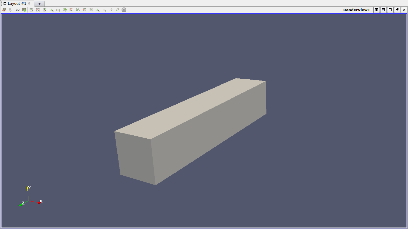
In each of them, we started from the exact solution T, calculated the conditions of Neumann, Dirichlet and Robin associated with this T, then launched the simulation on a geometry representing a bar, which is as follows:
In each case we used as exact solution the function \(T=x^2yzt\). By injecting into the equation we find that the source term is \(f=C_p\rho x^2yz-2kyzt\).
The first case consists in considering Dirichlet conditions on the \(z=0\) side and Neumann conditions on the other sides, in order to test the Neumann and Dirichlet conditions.
This is the associated json file :
{
    "Name": "Heatonly",
    "ShortName":"HO",
    "Models":"mythermicmodel",
    "Parameters":
    {
        "k":"393", //[W/(m*K)]
        "Cp":"386.e+06", //[J/(kg/K)]
        "rho":"8.94e-09" //[kg/(m^3)]
    },
    "Materials":
    {
        "Omega":
        {
            "name":"mymat1",
            "physics":["heat"],
            "k":"393", //[W/(m*K)]
            "Cp":"386.e+06", //[J/(kg/K)]
            "rho":"8.94e-09" //[kg/(m^3)]
        }
    },
    "BoundaryConditions":
    {
        "temperature":
        {
            "SourceTerm":
            {
                "Omega":
                {
                    "expr":"y*z*((386.e+06)*(8.94e-09)*x*x-393*2*t):x:y:z:t"
                }
            },
            "Dirichlet":
            {
                "Dirichlet":
                {
                    "expr":"x*x*y*z*t:x:y:z:t"
                }
            },
            "Neumann":
            {
                "Neumann1":
                {
                    "expr":"-393*(2*x*y*z*t*nx+x*x*z*t*ny+x*x*y*t*nz):x:y:z:t:nx:ny:nz"
                },
                "Neumann2":
                {
                    "expr":"-393*(2*x*y*z*t*nx+x*x*z*t*ny+x*x*y*t*nz):x:y:z:t:nx:ny:nz"
                },
                "Neumann3":
                {
                    "expr":"-393*(2*x*y*z*t*nx+x*x*z*t*ny+x*x*y*t*nz):x:y:z:t:nx:ny:nz"
                },
                "Neumann4":
                {
                    "expr":"-393*(2*x*y*z*t*nx+x*x*z*t*ny+x*x*y*t*nz):x:y:z:t:nx:ny:nz"
                },
                "Neumann5":
                {
                    "expr":"-393*(2*x*y*z*t*nx+x*x*z*t*ny+x*x*y*t*nz):x:y:z:t:nx:ny:nz"
                }
            }
        }
    },
    "PostProcess":
    {
        "Exports":
        {
            "fields":["temperature"]
        }
    }
}
Config file, json file and geo file are stored in src/cases/heat/ in the heat branch, and are named heatonly.xxx.
You can run the simulation by using :
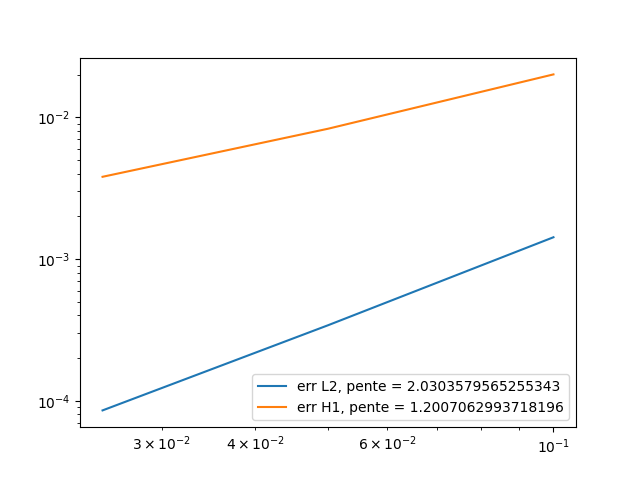
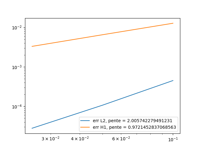
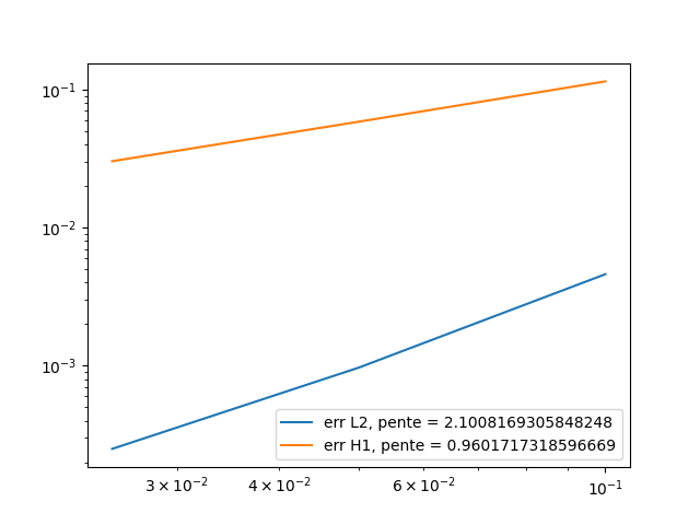
mpirun -np 8 feelpp_mqs_heat --config-file cases/heat/heatonly.cfg --gmsh.hsize=0.025 --pc-type gasm --ksp-monitor=1To check if the code is correct, we check the order of \(L^2\) and \(H^1\) errors.
Below are the errors we get at different times, with the associated graph in log scale.
\(t=0.1\):
h |
0.1 |
0.05 |
O.0025 |
\(L^2\) error |
0.001426 |
0.000341 |
8.5452e-05 |
\(H^1\) error |
0.020129 |
0.008321 |
0.00381 |
\(t=0.5\):
h |
0.1 |
0.05 |
O.0025 |
\(L^2\) error |
0.007329 |
0.00176 |
0.000442 |
\(H^1\) error |
0.100685 |
0.04160 |
0.019687 |

\(t=0.9\):
h |
0.1 |
0.05 |
O.0025 |
\(L^2\) error |
0.013260 |
0.00319 |
0.00080 |
\(H^1\) error |
0.181243 |
0.07498 |
0.03435 |

As we can see, the orders of the errors are close to those expected, the solution converges well towards the exact solution. So the calculation of Neumann’s and Dirichlet’s terms works.
The second case consists in considering Robin conditions on the \(z=5\) side and Dirichlet conditions on the other sides, in order to test the Robin (and Dirichlet) conditions.
This is the associated json file :
{
    "Name": "Heatonly",
    "ShortName":"HO",
    "Models":"mythermicmodel",
    "Parameters":
    {
        "k":"393", //[W/(m*K)]
        "Cp":"386.e+06", //[J/(kg/K)]
        "rho":"8.94e-09" //[kg/(m^3)]
    },
    "Materials":
    {
        "Omega":
        {
            "name":"mymat1",
            "physics":["heat"],
            "k":"393", //[W/(m*K)]
            "Cp":"386.e+06", //[J/(kg/K)]
            "rho":"8.94e-09" //[kg/(m^3)]
        }
    },
    "BoundaryConditions":
    {
        "temperature":
        {
            "SourceTerm":
            {
                "Omega":
                {
                    "expr":"y*z*((386.e+06)*(8.94e-09)*x*x-393*2*t):x:y:z:t"
                }
            },
            "Dirichlet":
            {
                "Dirichlet":
                {
                    "expr":"x*x*y*z*t:x:y:z:t"
                }
            },
            "Robin":
            {
                "Robin":
                {
                    "expr1":"4.35e-03",
                    "expr2":"x*x*y*z*t + (393/4.35e-03)*(2*x*y*z*t*nx+x*x*z*t*ny+x*x*y*t*nz):x:y:z:t:nx:ny:nz"
                }
            }
        }
    },
    "PostProcess":
    {
        "Exports":
        {
            "fields":["temperature"]
        }
    }
}
Config file, json file and geo file are stored in src/cases/heat/ in the heat branch, and are nammed heatonlyrobin.xxx.
You can run the simulation by using :
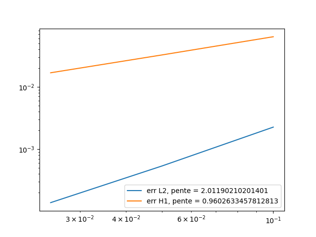
mpirun -np 8 feelpp_mqs_heat --config-file cases/heat/heatonlyrobin.cfg --gmsh.hsize=0.025 --pc-type gasm --ksp-monitor=1To check if the code is correct, we check the order of \(L^2\) and \(H^1\) errors.
Below are the errors we get at different times, with the associated graph in log scale.
\(t=0.1\):
h |
0.1 |
0.05 |
O.0025 |
\(L^2\) error |
0.00045 |
0.000107 |
2.7902e-05 |
\(H^1\) error |
0.01270 |
0.00650 |
0.00330 |
\(t=0.5\):
h |
0.1 |
0.05 |
O.0025 |
\(L^2\) error |
0.002261 |
0.000538 |
0.000139 |
\(H^1\) error |
0.063674 |
0.032501 |
0.016820 |
\(t=0.9\):
h |
0.1 |
0.05 |
O.0025 |
\(L^2\) error |
0.00460 |
0.000969 |
0.000250 |
\(H^1\) error |
0.11461 |
0.058510 |
0.030279 |
As we can see, the orders of the errors are also close to those expected, the solution converges well towards the exact solution. So the calculation of Robin’s terms works.
4. MQS with heat equation
First, let’s remember the two equations of the MQS model :
where :
-
\(A\) is the magnetic potential
-
\(V\) is the scalar electric potential
-
\(\mu_0(r,t)\) is the permeability of vaccum
-
\(\sigma(r,t)\) is the conductivity
We now wish to add the heat equation to the two equations of the mqs model. For this, the source term of the heat equation will be joule losses, defined by :
so the heat part will be :
Finally we have the system :
Now, adding the weak formulation of the formulation section with the heat weak formulation, we have :
5. Resolution Strategy
As we can see, the second member of the heat equation is non-linear. Therefore, a different resolution strategy must be adopted than previously.
The first possibility is to first solve the MQS equations and then solve the heat equation. This can be interesting in the case where the parameters of the equations do not depend on temperature.
Another option is to solve the two equations again separately, but by approaching the non-linear terms of the heat equation with a fixed point method, e.g. picard. Alternatively, a relaxation parameter can be added,\(\alpha\). If \(T_{new}\) is the solution obtain with picard, and \(T_{old}\) the old one, we evaluate the equation in \((1-\alpha)T_{new}+\alpha T_{old}\).
The last possibility is to solve the three equations at the same time, as a block, by adding a time loop to apply a fixed point and relaxation method on the heat part.