Implementation of MQS equations and results

1. Implementation

Here are the important points of the code that solves the MQS system of equations in our test cases. The file is called "mqs-form.cpp" in the master branch.

We first define our function spaces Ah and Vh, as well as A and V on their respective space :

  auto Ah = Pchv<1>( mesh );
  auto Vh = Pch<1>( mesh, markedelements(mesh, range) );

  auto A = Ah->elementPtr();
  auto V = Vh->elementPtr();

We then initialize A and V by A0 and V0 given :

  auto A0 = expr<3, 1>(soption(_name="A0"));
  auto V0 = expr(soption(_name="V0"));
  (*A) = project(_space = Ah, _expr = A0);
  (*V) = project(_space = Vh, _expr = V0);

We then define our "blocks" where we will store our equations. The block structure consists of transforming our system of equations into the form \(MU=F\) where U is the desired vector.

  BlocksBaseGraphCSR myblockGraph(2,2);
  myblockGraph(0,0) = stencil(_test=Ah,_trial=Ah, _diag_is_nonzero=false, _close=false)->graph();
  myblockGraph(0,1) = stencil(_test=Ah,_trial=Vh, _diag_is_nonzero=false, _close=false)->graph();
  myblockGraph(1,0) = stencil(_test=Vh,_trial=Ah, _diag_is_nonzero=false, _close=false)->graph();
  myblockGraph(1,1) = stencil(_test=Vh,_trial=Vh, _diag_is_nonzero=false, _close=false)->graph();
  auto M = backend()->newBlockMatrix(_block=myblockGraph);

  BlocksBaseVector<double> myblockVec(2);
  myblockVec(0,0) = backend()->newVector( Ah );
  myblockVec(1,0) = backend()->newVector( Vh );
  auto F = backend()->newBlockVector(_block=myblockVec, _copy_values=false);

  BlocksBaseVector<double> myblockVecSol(2);
  myblockVecSol(0,0) = A;
  myblockVecSol(1,0) = V;
  auto U = backend()->newBlockVector(_block=myblockVecSol, _copy_values=false);

We then implement our equations as well as the boundary conditions :

  for (t = dt; t < tmax; t += dt)
  {
    auto M00 = form2( _trial=Ah, _test=Ah ,_matrix=M, _rowstart=0, _colstart=0 );
    for( auto const& pairMat : M_modelProps->materials() )
	  {
	    auto name = pairMat.first;
	    auto material = pairMat.second;
	    auto mur = material.getScalar("mu_mag");

	    M00 += integrate( _range=markedelements(mesh, material.meshMarkers()),
			                  _expr = dt * 1/mur * trace(trans(gradt(A))*grad(A)) );
	  }

    auto M01 = form2( _trial=Vh, _test=Ah ,_matrix=M, _rowstart=0, _colstart=1 );
    auto F0 = form1( _test=Ah, _vector=F, _rowstart=0 );
    auto M11 = form2( _trial=Vh, _test=Vh ,_matrix=M, _rowstart=1, _colstart=1 );
    auto M10 = form2( _trial=Ah, _test=Vh ,_matrix=M, _rowstart=1, _colstart=0 );
    auto F1 = form1( _test=Vh ,_vector=F, _rowstart=1 );

    for( auto const& pairMat : M_materials )
	  {
	    auto name = pairMat.first;
	    auto material = pairMat.second;
	    auto sigma = material.getScalar("sigma");

	    M00 += integrate(_range=markedelements(mesh, material.meshMarkers()),
			                 _expr = mu0 * sigma * inner(id(A) , idt(A) ));

	    M01  += integrate(_range=markedelements(mesh, material.meshMarkers()),
			                  _expr = dt * mu0 * sigma * inner(id(A),trans(gradt(V))) );

	    F0 += integrate(_range=markedelements(mesh, material.meshMarkers()),
			                _expr = mu0 * sigma * inner(id(A) , idv(Aold)));

	    M11 += integrate(_range=markedelements(cond_mesh, material.meshMarkers()),
			                 _expr = mu0 * sigma * dt * inner(gradt(V), grad(V)) );

	    M10 += integrate(_range=markedelements(cond_mesh, material.meshMarkers()),
			                 _expr = mu0 * sigma * inner(idt(A), trans(grad(V))) );

	    F1 += integrate(_range=markedelements(cond_mesh, material.meshMarkers()),
			                _expr = mu0 * sigma * inner(idv(Aold), trans(grad(V))) );
	  }
    auto itField = M_modelProps->boundaryConditions().find( "magnetic-potential");
    if ( itField != M_modelProps->boundaryConditions().end() )
	  {
	    auto mapField = (*itField).second;
	    auto itType = mapField.find( "Dirichlet" );
	    if ( itType != mapField.end() )
	    {
	      for ( auto const& exAtMarker : (*itType).second )
		    {
		      std::string marker = exAtMarker.marker();
		      auto g = expr<3,1>(exAtMarker.expression());
		      g.setParameterValues({{"t", t}});
		      M00 += on(_range=markedfaces(mesh,marker), _rhs=F, _element=*A, _expr= g);
		    }
	    }
	    itType = mapField.find( "DirichletX" );
	    if ( itType != mapField.end() )
	    {
	      for ( auto const& exAtMarker : (*itType).second )
		    {
		      std::string marker = exAtMarker.marker();
		      auto g = expr(exAtMarker.expression());
		      g.setParameterValues({{"t", t}});
		      M00 += on(_range=markedfaces(mesh,marker), _rhs=F, _element=(*A)[Component::X], _expr= g);
		    }
	    }
	    itType = mapField.find( "DirichletY" );
	    if ( itType != mapField.end() )
	    {
	      for ( auto const& exAtMarker : (*itType).second )
		    {
		      std::string marker = exAtMarker.marker();
		      auto g = expr(exAtMarker.expression());
		      g.setParameterValues({{"t", t}});
		      M00 += on(_range=markedfaces(mesh,marker), _rhs=F, _element=(*A)[Component::Y], _expr= g);
		    }
	    }
	    itType = mapField.find( "DirichletZ" );
	    if ( itType != mapField.end() )
	    {
	      for ( auto const& exAtMarker : (*itType).second )
		    {
		      std::string marker = exAtMarker.marker();
		      auto g = expr(exAtMarker.expression());
		      g.setParameterValues({{"t", t}});
		      M00 += on(_range=markedfaces(mesh,marker), _rhs=F, _element=(*A)[Component::Z], _expr= g);
		    }
	    }
	  }
    itField = M_modelProps->boundaryConditions().find( "electric-potential");
    if ( itField != M_modelProps->boundaryConditions().end() )
	  {
	    auto mapField = (*itField).second;
	    auto itType = mapField.find( "Dirichlet" );
	    if ( itType != mapField.end() )
	    {
	      for ( auto const& exAtMarker : (*itType).second )
		    {
		      std::string marker = exAtMarker.marker();
		      auto g = expr(exAtMarker.expression());
		      g.setParameterValues({{"t", t}})
		      M11 += on(_range=markedfaces(cond_mesh,marker), _rhs=F, _element=*V, _expr= g);
		    }
	    }
	  }
    ...
  }

Finally, the system is solved by calculating U containing A and V, and then the following time step is carried out.

    auto result = mybackend->solve( _matrix=M, _rhs=F, _solution=U, _rebuild=true);

2. Results

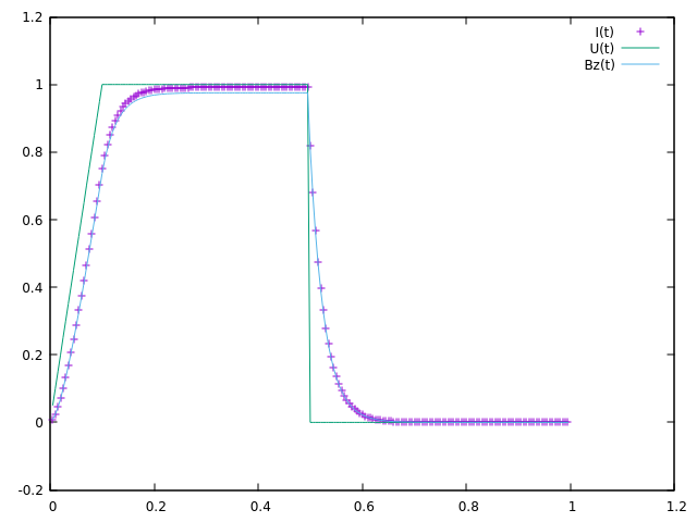
2.1. A solenoidal magnet

The normalized computed electric potential, current and magnetic field at the Origin are plotted bellow:

results

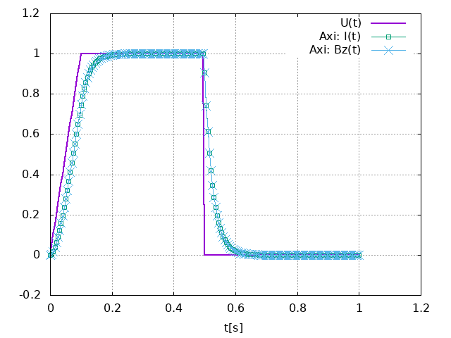
We use the expected values of the applied electric potential, current and magnetic field for the transient regime (aka t):

	Value	Unit
\(V\)	1	V
\(I\)	135069	A
\(B_z(\mathbf{O})\)	0.944	T

Value

Unit

\(V\)

\(I\)

135069

\(B_z(\mathbf{O})\)

0.944

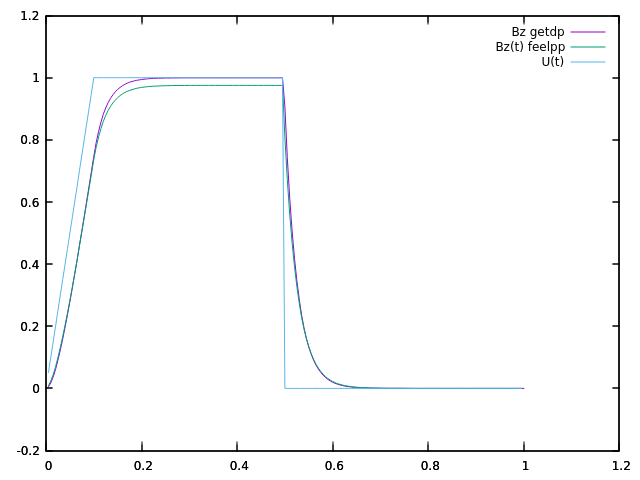
Here is what we get on feelpp using the block-form program, after normalization by the above values.

results

To obtain these results, use the command :

mpirun -np 1 feelpp_mqs_form --config-file cases/quart-turn/quart-turn.cfg --gmsh.hsize 0.05 --pc-type gasm --ksp-monitor=1

This will produce a csv file in the feel folder associated with this case.

Below is the comparison between getdp and feelpp result :

results

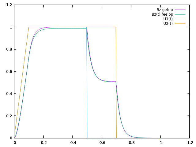
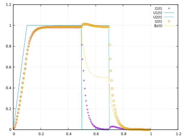
2.2. 2 solenoidal magnets

The normalized computed electric potential, current and magnetic field at the Origin are plotted bellow:

results

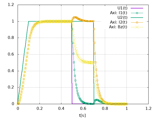
We use the expected values of the applied electric potential, current and magnetic field for the transient regime (aka t):

	Value	Unit
\(V\)	1	V
\(I\)	135069	A
\(B_z(\mathbf{O})\)	0.850698279	T

Value

Unit

\(V\)

\(I\)

135069

\(B_z(\mathbf{O})\)

0.850698279

Here is what we get on feelpp using the block-form program, after normalization by the above values.

results

To obtain these results, use the command :

mpirun -np 1 feelpp_mqs_form --config-file cases/quart-turn/quart-turn2.cfg --gmsh.hsize 0.05 --pc-type gasm --ksp-monitor=1

This will produce a csv file in the feel folder associated with this case.

Below is the comparison between getdp and feelpp result :

results