Validations
1. Introduction
Two simple test cases are used to validate the formulation:
-
a single magnet,
-
a set of 2 magnets.
We will consider simple geometries for the magnets. They are modeled as rectangular cross section torus. This allows us to derive analytical expressions for the resistance \(R\) and inductances \(L\) of the magnets. For each case, we will model the powering and a powerfailure. The computed total current flowing into the magnets will be compared to the results obtained by a simple equivalent \(RL\) circuit. The circuit may be either modeled by a simple ODE solver or using analytical methods (aka exponential Matrices). For other quantities, we will compared our simulation results with other Finite Element Solver. We have chosen getdp with a MQS formulation for axisymetric geometries.
NB: getdp model and test geometry are accessible here. To reproduce the results follow the procedure in this appendix.
2. A solenoidal magnet
2.1. Setup
The magnet is centered on the origin of the cylindrical frame as shown bellow.
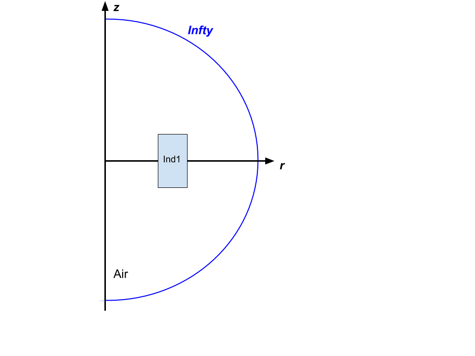
The geometry is defined by the following parameters:
| Name | Description | Value | Unit |
|---|---|---|---|
\(r_i\) |
internal radius |
75. |
\(mm\) |
\(r_e\) |
external radius |
100.2 |
\(mm\) |
\(h\) |
heigth |
50. |
\(mm\) |
\(r_\text{infty}\) |
internal radius |
500. |
\(mm\) |
The magnet is supposed to be made of some conducting amagnetic material:
| Name | Description | Marker | Value | Unit |
|---|---|---|---|---|
\(\sigma\) |
electric conductivity |
Ind |
\(58.e3\) |
\(S.mm^{-1}\) |
\(\mu_r\) |
relative magnetic permeability |
Ind |
\(1\) |
The applied source electrical potential has the following form:
| \(V_D\) | electrical potential | \(1*t/(0.1*\tau)\) | \(V\) | \(0 <= t < 0.1\,\tau\) |
|---|---|---|---|---|
\(V_D\) |
electrical potential |
1 |
\(V\) |
\( 0.1 \, \tau <= t <= 0.5\,\tau\) |
\(V_D\) |
electrical potential |
0 |
\(V\) |
\(t>\tau\) |
The boundary conditions for the electromagnetic problem are:
| Marker | Type | Value |
|---|---|---|
\(Oz\) Axis |
Dirichlet |
\(\mathbf{0}\) |
Infty |
Dirichlet |
\(\mathbf{0}\) |
2.2. Resistance \(R\) and Self Inductance \(L\)
The resistance is defined as the ration of the applied electrical potential difference over the total current. In case of a rectangular cross section \( (r_1,r_2) \times (z_1,z_2) \) torus, we can show that:
with \(\rho=1/\sigma\) the resistivity of the material composing the torus. For details on this expression, see feelpp electric toolbox test case.
As for the self-inductance, we recall the defintion of the stored magnetic energy:
to continue…
2.3. Equivalent circuit model
From a macroscopic point of view, the studied system is simply equivalent to a \(RL\) circuit modeled by:
| Value | Unit | |
|---|---|---|
\(R\) |
\(7.5313 10^{-6}\) |
Ohm |
\(L\) |
\(1.9204 10^{-7}\) |
Henry |
2.4. Results
The normalized computed electric potential, current and magnetic field at the Origin are plotted bellow:
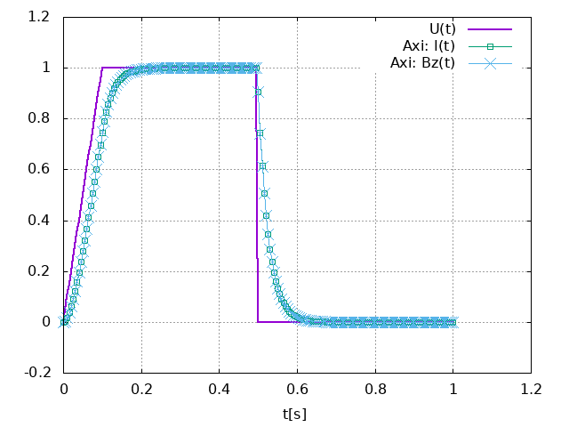
We use the expected values of the applied electric potential, current and magnetic field for the transient regime (aka t):
| Value | Unit | |
|---|---|---|
\(V\) |
1 |
V |
\(I\) |
135069 |
A |
\(B_z(\mathbf{O})\) |
0.944 |
T |
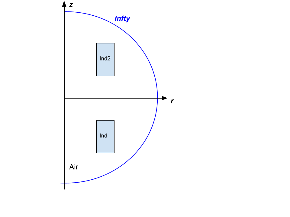
3. 2 solenoidal magnets
For sake of simplicity, we consider 2 solenoid magnets similar to the one described in previous section stacked as shown bellow.
insert a figure
3.1. Mutual Inductance \(M\)
Obviously, the 2 magnets have the same resistance and self-inductance as they have the same geometry and are made of the same material. We only need then to compute the so-called mutual inductance \(M\).
As before, we start wih the stored magnetic energy \(E\) of the system:
to continue…
3.2. Equivalent circuit model
The equivalent circuit is this time similar to a transformer circuit. Thus, it may be modeled as:
In our case, we have \(R_1=R_2\) and \(L_1=L_2\).
| Value | Unit | |
|---|---|---|
\(R\) |
\(7.5313 10^{-6}\) |
Ohm |
\(L\) |
\(1.9204 10^{-7}\) |
Henry |
\(M\) |
\(2.6487 10^{-8}\) |
Henry |
3.3. Results
The normalized computed electric potential, current and magnetic field at the Origin are plotted bellow:
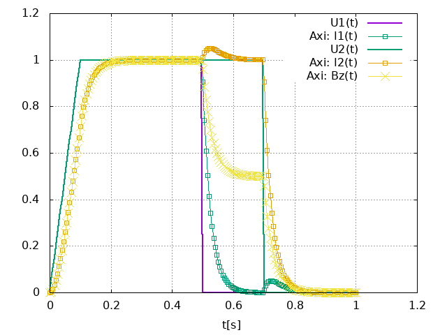
We use the expected values of the applied electric potential, current and magnetic field for the transient regime (aka t):
| Value | Unit | |
|---|---|---|
\(V\) |
1 |
V |
\(I\) |
135069 |
A |
\(B_z(\mathbf{O})\) |
0.8507 |
T |