Eye2Brain Level 2 Application
Eye2brain Level 2 is in two parts :
-
poroelastic model solved in the lamina cribrosa, coupled with the retinal blood circulation developed in OpenModelica.
-
poroelastic model solved in the lamina cribrosa, coupled with the retinal blood circulation developed in OpenModelica and the biomechanical behavior of the retina, choroid, retina and cornea. This case is not yet documented in this document.
1. Model
The hemodynamics of the lamina cribrosa is the same as Level 1, and for what concerns the three-dimensional description of the tissue in this case we add also the linear elastic system in order to simulate the poroelastic behaviour of the lamina cribrosa.
The input data are the intraocular pressure (IOP), the retrolamina tissue pressure (RLTp), the blood pressure standard measurements and the material properties of the lamina cribrosa. The simulation domain is a simple geometrical description of the lamina cribrosa realized with Gmsh, where the dimensions are taken from baseline values present in literature.
The system is discretized using the hybridizable discontinuous Galerkin (HDG) method and it is solved numerically adopting a static condensation technique to boost the computational performances.
2. Input
The input of this model are
-
the intraocular pressure (IOP) that is modelled as a ramp voltage source;
-
the retrolaminar tissue pressure (RLTp) that is represented by a constant voltage source;
-
the central retina artery (CRA) pressure that is characterized by a voltage source and it is univocally defined by the heart rate (HR), the systolic blood pressure (SBP) and diastolic blood pressure (DBP).
-
the CRV pressure that infer on the internal lateral boundary for the Darcy problem (CRVp)
-
the CRA pressure that infer on the internal lateral boundary for the elastic problem (CRAp)
[eye2brain]
level2=true
# circuit data
IOP=16.0
RLTp=7.0
HR=60
SBP=120
DBP=80
# Poisson data
CRVp=19
CRVp_marker=Hole
# Elasticity data
CRAp=80
IOP_marker=Lamina_Retina
RLTp_marker=Out
CRAp_marker=Hole-
the material properties for the porous part
    "Materials":
    {
        "Lamina":
        {
            "name":"tissue",
            "k":"0.015192",
            "Lamina_Sclera-buffer":"C5.p.v",
            "Cbuffer_name":"C5",
            "Rbuffer_name":"lcRin"
        }
},-
the material properties for the elastic part
    "Materials":
    {
        "Lamina":
        {
            "name":"tissue",
            "rho":"0.0011",
            "lambda":"588 * 10^(-2)",
            "mu":"12 * 10^(-2)",
            "special_neumann":"Hole",
            "scale_stress":"10^2"
        }
},-
the simulation geometry
h=0.1;


Point(1) = {0.095, 0, -0.015, h};
Point(2) = {0, 0, -0.015, h};
Point(3) = {0.04750000000000001, 0.08227241335952167, -0.015, h};
Point(4) = {-0.08227241335952169, -0.04749999999999997, -0.015, h};
Point(5) = {0.008, 0, -0.015, h};
Point(6) = {0, 0.008, -0.015, h};
Point(7) = {-0.008, 0, -0.015, h};
Point(8) = {0, -0.008, -0.015, h};
Point(9) = {0.095, 0, 0.015, h};
Point(10) = {0, 0, 0.015, h};
Point(11) = {0.04750000000000001, 0.08227241335952167, 0.015, h};
Point(14) = {-0.08227241335952169, -0.04749999999999997, 0.015, h};
Point(15) = {0, 0.008, 0.015, h};
Point(17) = {0.008, 0, 0.015, h};
Point(20) = {0, -0.008, 0.015, h};
Point(23) = {-0.008, 0, 0.015, h};
Circle(1) = {1, 2, 3};
Circle(2) = {3, 2, 4};
Circle(3) = {4, 2, 1};
Circle(5) = {5, 2, 6};
Circle(6) = {6, 2, 7};
Circle(7) = {7, 2, 8};
Circle(8) = {8, 2, 5};
Circle(9) = {9, 10, 11};
Line(10) = {1, 9};
Line(11) = {3, 11};
Circle(13) = {11, 10, 14};
Line(15) = {4, 14};
Circle(17) = {14, 10, 9};
Circle(21) = {15, 10, 17};
Line(22) = {6, 15};
Line(23) = {5, 17};
Circle(25) = {17, 10, 20};
Line(27) = {8, 20};
Circle(29) = {20, 10, 23};
Line(31) = {7, 23};
Circle(33) = {23, 10, 15};
Line Loop(12) = {1, 11, -9, -10};
Ruled Surface(12) = {12};
Line Loop(16) = {2, 15, -13, -11};
Ruled Surface(16) = {16};
Line Loop(20) = {3, 10, -17, -15};
Ruled Surface(20) = {20};
Line Loop(24) = {-5, 23, -21, -22};
Ruled Surface(24) = {24};
Line Loop(28) = {-8, 27, -25, -23};
Ruled Surface(28) = {28};
Line Loop(32) = {-7, 31, -29, -27};
Ruled Surface(32) = {32};
Line Loop(36) = {-6, 22, -33, -31};
Ruled Surface(36) = {36};
Line Loop(1000) = {1, 2, 3, 6, 7, 8, 5};
Plane Surface(1000) = {1000};
Line Loop(1001) = {9, 13, 17, -33, -29, -25, -21};
Plane Surface(1001) = {1001};
Surface Loop(3000) = {12, 16, 20, 24, 28, 32, 36, 1000, 1001};
Volume(3000) = {3000};

// Physical labels
Physical Surface("Lamina_Sclera") = {12, 16, 20}; // Integral
Physical Surface("Out") = {1000} ; // Neumann
Physical Surface("Lamina_Retina") = {1001} ; // Neumann
Physical Surface("Hole") = {24, 28, 32, 36}; // Dirichlet
Physical Volume("Lamina") = {3000};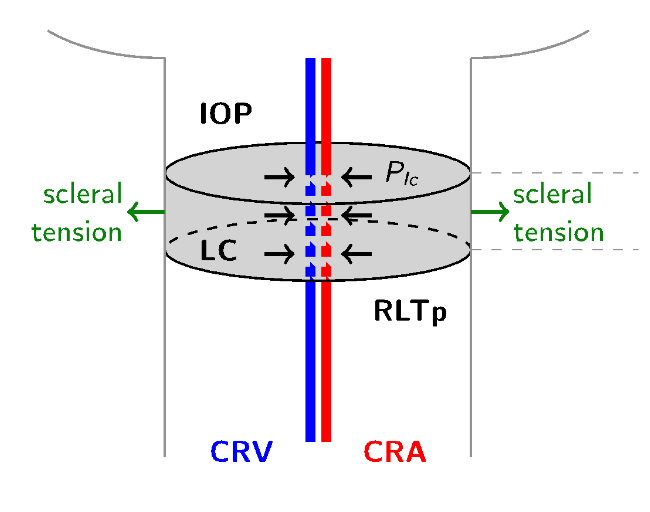
3. Outputs
Currently available outputs in Feel model:
-
blood velocities in retinal circulation. Those values are exported in a [time,value]
.csvfile. For example the blood velocity in CRA/CRV. -
3D visualization (through Paraview) of the discharge velocity and pressure fields. From those fields, all derived quantities can be retrieved, for example the mean pressure on the interface between lamina and sclera.
-
3D visualization (through Paraview) of the displacement and stress tensor.
5. Advanced Usage
5.1. Advanced Numerical Inputs
The configuration of the model is made through 3 input files :
-
the
.cfgfile contains the configuration of the model (tipe step, mesh size, solver configuration, …) -
the
.jsonfile contains the physical parameters and a description of the boundary conditions of the model -
the
.geoor.mshfile contains the geometry description or the mesh of the computation domain.
Here is a non-exhaustive list of inputs that can be modified in the .cfg file :
-
gmsh.filename: the.geo,.mshor.json/.h5file used to describe the domain -
gmsh.hsize: characteristic length used to generate the mesh from.geofile -
gmsh.submesh: submesh where the Poisson equation has to be solved -
mixedelasticity.gmsh.submesh: submesh where the elastic problem has to be solved -
mixedpoisson.filename: the.jsonfile used to describe the model -
mixedelasticity.filename: the.jsonfile used to describe the model -
bdf.order: order of the time discretization method -
bdf.ts.time-step: time step of the time discretization algorithm
Here is a list of the principal features defined in the .json file :
-
Materials: definition of domain properties (e.g.kis the permeability coefficient) -
Potential: definition ofInitialSolution,SourceTerm,Dirichletboundary condition andNeumannboundary condition -
Flux: definition of theIntegralboundary condition -
stress: definition of 'SourceTerm' and 'Neumann` boundary condition -
displacement: definition ofDirichletboundary condition -
ExactSolution: definition of the exact solution (if any) to which compare the numerical outcomes -
PostProcess: definition of exported quantities