Tools
1. Python libraries
Created by the Google Brain team, TensorFlow is an open source library for numerical computation and large-scale machine learning. TensorFlow bundles together a slew of machine learning and deep learning.
It is a programming system in which the calculations are represented graphically. The nodes of the graph represent mathematical operations, and the borders represent arrows of multidimensional data communicated between them, creating so-called tensors. It is particularly suitable for very large-scale parallel processing applications : neural networks. Tansorflow was open sourced in November 2015, and version 2.0 was released in 2019.
Created in 2007, scikit-learn is an open-source library for the machine learning in Python. Benefiting from an extremely active community, it gathers all the main algorithms of machine learning(classification, regression,…). It is designed to harmonize with other open-source libraries, including NumPy and SciPy.
Keras is a high-level neural network API written in Python and interfaces with TensorFlow, Microsoft Cognitive Toolkit (CNTK) and Theano. It is designed to be modular, fast and easy to use.
2. Activation functions
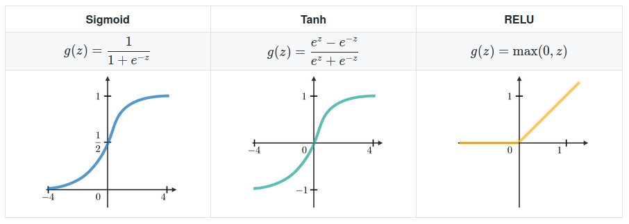
The activation function makes the decision whether or not to transmit the signal. It transforms the signal to obtain an output value from complex transformations between inputs. To do this, the activation function must be non-linear because it allows non-linear separable data. Linear functions only work with a single neuron layer, beyond one layer the recurrent application of the same linear activation function will have no impact on the result. The most used non-linear functions are the following :
3. Loss functions
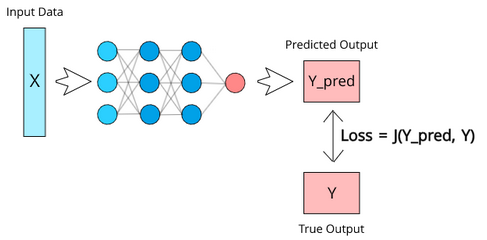
The loss function is a method for assessing the quality of data modeling by a specific algorithm. If the predictions deviate too much from the actual results, the loss function would spit out a very large number of them. It takes into account two parameters : the predicted output and the actual output (cf. [Loss]).
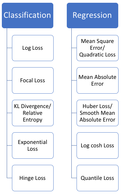
There is no single loss function for algorithms in machine learning. Different factors are involved in the choice of a loss function for a specific problem, such as the type of machine learning algorithm chosen, the ease of calculating derivatives, and to some extent the percentage of outliers in the data set.
The most popular loss functions currently in use in relation to the type of problem are as follows (cf. [Lossfunctions]) :
-
Mean square error(MSE) : is measured as the mean square of the difference between predictions and actual observations. Because of the square, predictions that are far from the actual values are heavily penalized compared to less deviant predictions.
\[MSE=\dfrac{\sum_{i=1}^n(y_i-\hat{y}_i)^2}{n}\]Where:
-
\(n\) : number of training examples.
-
\(y_i\) : ground truth label for the ith training example.
-
\(\hat{y}_i\) : prediction for the ith training example.
-
-
Root mean square error (RMSE) : is the square root of MSE .
\[RMSE=\sqrt{MSE}\] -
Mean absolute error (MAE) : is measured as the average of sum of absolute differences between predictions and actual observations. MAE is more robust to outliers since it does not make use of square.
\[MAE=\dfrac{\sum_{i=1}^n|y_i-\hat{y}_i|}{n}\]Where:
-
\(n\) : number of training examples.
-
\(y_i\) : ground truth label of the ith training example.
-
\(\hat{y}_i\) : prediction of the ith training example.
-
-
Huber or Smooth Mean Absolute Error : It’s basically absolute error, which becomes quadratic when error is small. It depends on a hyper-parameter \(\delta\). Huber loss approaches MAE when \(\delta \sim 0\), and approaches MSE when \(\delta \sim \infty\).
\[L_\delta (y,\hat{y})= \left\lbrace \begin{array}{cl} \dfrac{1}{2}(y-\hat{y})^2& for|y-\hat{y}|\leq \delta \\ \delta |y-\hat{y}|-\dfrac{1}{2} \delta^2 & otherwise \end{array} \right.\]Where:
-
\(y\) : ground truth label of the training example.
-
\(\hat{y}\) : prediction of the training example.
-
-
Log-Cosh Loss : is the logarithm of the hyperbolic cosine of the prediction error.
\[L (y,\hat{y})=\sum_{i=1}{n}\log(cosh(\hat{y}-y))\]Where:
-
\(y\) : ground truth label of the training example.
-
\(\hat{y}\) : prediction of the training example.
-
-
Cross-entropy loss(log loss) : measures the performance of a classification model whose output is a probability value between 0 and 1. A perfect model would have a log loss of 0.
\[CE= \left\lbrace \begin{array}{cl} −(y\log(p)+(1−y)\log(1−p))& if M=2 \\ -\sum_{i=1}^{M}y_{o,c}\log(p_{o,c}) & if M>2 \end{array} \right.\]Where:
-
M : number of classes.
-
y : binary indicator (0 or 1) if class label c is the correct classification for observation o.
-
p : predicted probability observation o is of class c.
-
-
Focal loss (FL) : is designed to meet the one-step object detection scenario, which there is an extreme imbalance between foreground and background classes during training.
The focus parameter \(\gamma\) smoothly adjusts the speed which easy examples are weighted down. When \(\gamma=0\). It is equivalent to Cross-entropy loss. When \(\gamma\) is increased, the effect of the modulation factor is also increased.
\[FL(p_t)=-(1-p_t)^\gamma log(p_t)\]\[p_t= \left\lbrace \begin{array}{cl} p& if y = 1 \\ 1-p & otherwise \end{array} \right.\]Where:
-
y : binary indicator (0 or 1) if class label \(c\) is the correct classification for observation \(o\).
-
p : predicted probability observation \(o\) of the class \(c\).
-
\(\gamma\) : focusing parameter.
-
-
Relative entropy (Kullback-Leibler divergence) : is a measure of the distance between two probability distributions on a random variable. Formally, given two probability distributions \(p(x)\) and \(q(x)\) over a discrete random variable X, the relative entropy is given by :
\[KL(p||q)=\sum_{x \in X}p(x) log(\dfrac{p(x)}{q(x)})\]
4. Gradient descent
Gradient Descent is the most basic but most widely used optimization algorithm in machine learning to reduce the cost function. It will help models to make accurate predictions. It is widely used in linear regression and classification algorithms. Reverse propagation in neural networks also uses a gradient descent algorithm.
This method has been used in many algorithms according to their specificities : gradient descent by batch, stochastic (SGD), mini-batch,…
The gradient descent is fast, efficient, robust and above all flexible. Indeed, it is used in many algorithms, from Deep Learning with neural networks to the more traditional Learning Machine.
5. Optimizer
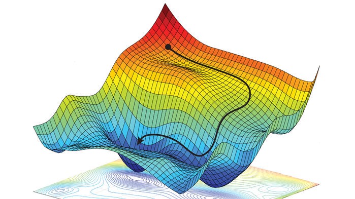
Optimizers update the weight parameters to minimize the loss function. Loss function acts as guides to the terrain telling optimizer if it is moving in the right direction to reach the bottom of the valley : the global minimum. The most commonly used optimizers are (cf. [Optimizers]) :
-
Momentum : it helps accelerate Gradient Descent (GD) when we have surfaces that curve more steeply in one direction than in another direction. For updating the weights, instead of using only the gradient of the current step to guide the search, momentum also accumulates the gradient of the past steps to determine the direction to go.
\[\begin{array}{cl} v_t \leftarrow & \gamma v_{t-1}+\eta \nabla_\theta J(\theta) \\ \theta \leftarrow & \theta-v_t \\ \end{array}\]With:
-
\(\gamma\) : coefficien of Momentum.
-
\(v_{t-1}\) : retained gradient.
-
\(\eta\) : learning rate.
-
\(\theta\) : weight parameter
-
-
Nesterov accelerated gradient(NAG) : is a method that consists of a gradient descent step, followed by something that looks a lot like a momentum term. NAG is like going down the hill and looking ahead in the future. This way, we can optimize our descent faster.
\[\begin{array}{cl} v_t \leftarrow & \gamma v_{t-1}+\eta \nabla_\theta J(\theta-\gamma v_{t-1}) \\ \theta \leftarrow & \theta-v_t \\ \end{array}\]Where:
-
\(\gamma\) : coefficien of Momentum.
-
\(v_{t-1}\) : retained gradient.
-
\(\eta\) : learning rate.
-
\(\theta\) : weight parameter
-
-
Adagra(Adaptive Gradient Algorithm) : is an adaptive learning rate method. It is well suited when we have sparse data as in large scale neural networks. GloVe word embedding uses adagrad where infrequent words required a greater update, and frequent words require smaller updates.
For SGD, Momentum, and NAG, we update for all parameters θ at once. We also use the same learning rate η. However, in Adagrad, we use different learning rate for every parameter θ for every time step t.
\[\begin{array}{cl} \theta_{t+1} =& \theta_t-\dfrac{\eta }{\sqrt{G_t + \epsilon}}.g_t\\ \end{array}\]With:
-
\(g_t=\nabla_\theta J(\theta_t)\)
-
\(G_{t}\) : contains the sum of the squares of the past gradients w.r.t. to all parameters θ along its diagonal.
-
\(\eta\) : learning rate.
-
\(\theta\) : weight parameter
-
-
Adadelta : is an extension of Adagrad that seeks to reduce its aggressive and monotonically decreasing learning rate.
\[\begin{array}{cl} \theta_{t} =& - \dfrac{RMS[\Delta \theta]_{t-1}}{RMS[g]_{t}}.g_t \\ \theta_{t+1}=& \theta_t + \Delta \theta_t \end{array}\]With:
-
\(g_t=\nabla_\theta J(\theta_t)\)
-
\(G_{t}\) : contains the sum of the squares of the past gradients w.r.t. to all parameters θ along its diagonal.
-
\(\theta\) : weight parameter.
-
\(\eta\) : learning rate.
-
RMS : root mean square
-
-
RMSProp(Root Mean Square Propogation) : was designed by the legendary Geoffrey Hinton. RMSProp attempts to solve Adagrad’s radically decreasing learning rates using a moving average of the square gradient. It uses the magnitude of recent gradient declines to normalize the gradient.
\[\begin{array}{cl} \theta_{t+1} =&\theta_t - \dfrac{\eta}{\sqrt{(1-\gamma)g^2_{t-1}+\gamma g_t +\epsilon}}.g_t \end{array}\]With:
-
\(g_t=\nabla_\theta J(\theta_t)\)
-
\(G_{t}\) : contains the sum of the squares of the past gradients w.r.t. to all parameters θ along its diagonal.
-
\(\eta\) : learning rate.
-
\(\gamma\) : the decay term that takes value from 0 to 1.
-
\(\theta\) : weight parameter.
-
-
Adam(Adaptative Momentum estimation) : can be seen as a combination of Adagrad, which works well on gentle gradients, RMSprop, and in online and non-stationary environments. It is the most widely used optimizer (especially for neural networks) because of its efficiency and stability.
\[\begin{array}{cl} v_{t} =&\beta_1 v_{t-1} -(1-\beta_1)g_t\\ s_{t} =&\beta_2 s_{t-1} -(1-\beta_2)g_t^2\\ \theta_{t+1}=&\theta_t - \eta \dfrac{v_t}{\sqrt{s_t+\epsilon}}g_t \end{array}\]With:
-
\(g_t=\nabla_\theta J(\theta_t)\)
-
\(v_t\) : exponential Average of gradients along \theta_j.
-
\(s_t\) : exponential Average of square of gradients along \theta_j.
-
\(\eta\) : learning rate.
-
\(\theta\) : weight parameter
-
The Hyperparameters \(\beta_1 \simeq 0.9\), \(\beta_2 \simeq 0.99 \) , \(\epsilon \simeq 1e-10\)
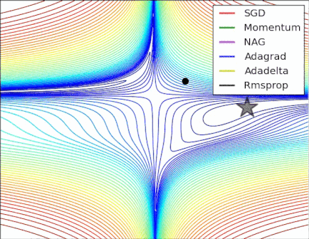 Figure 6. The different optimizer on loss surface contours(cf. [optimizeIA])
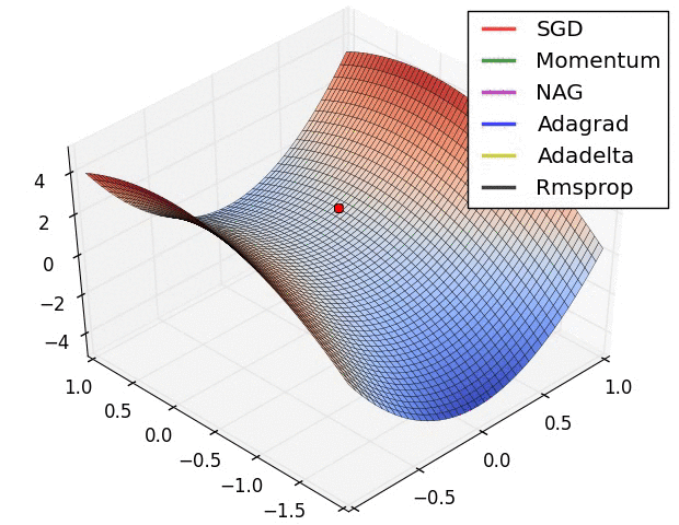 Figure 7. The different optimizer on saddle point(cf. [Optimizers])
 -
6. Scaling
Most of the time, in machine learning, the data sets come with different orders of magnitude which can lead to lower performance. Scaling can avoid this type of problem.
Scaling is a technique that is often applied when preparing data for the Machine Learning. Its objective is to change the numerical values in the data set to use a common scale, without the differences in the range of values being distorted and without loss of information. So that a significant number does not have an impact on the model solely because of their large magnitude.
Scaling makes algorithms such as neural network gradient descent converge much faster.
The most common techniques for feature scaling are :
-
normalization : is used to limit the values between two numbers, usually between [0,1] or [-1,1].
-
standardization : transform the data to have zero mean and a variance of 1, they make our data unitless.
6.1. Feature scaling methods
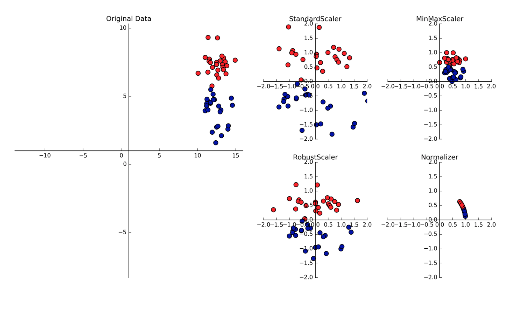
There are several ways in which we can scale the features, among them :
-
Min Max Scaler
This estimator scales and translates each feature individually so that it lies within the given range on the training set [0.1], or [-1.1] if it contains negative values.
This scaler responds well if the standard deviation is small and when a distribution is not Gaussian and it is sensitive to outliers.
\[x_{normalize}=\dfrac{x-x_{min}}{x_{max}-x_{min}}\]Where :
-
\(x_{min}\) : the smallest value observed for feature X
-
\(x_{max}\) : the highest observed value for the feature X
-
\(x\) : the value of the feature we want to normalize.
-
-
Standard Scaler
It scales so that the distribution is centered around 0, with a standard deviation of 1. Centering and scaling is done independently for each feature. If the data is not normally distributed, this is not the best scaler to use.
\[x_{normalize}=\dfrac{x-\mu}{\sigma}\]Where :
-
\(x\) : the value you want to standardise
-
\(\mu\) : the mean of the observations for this feature.
-
\(\sigma\) : the Standard Deviation of the observations for this feature.
-
-
Normalizer
This estimator applies by default the normalization L2 (can be replaced by L1) to each observation, so that the values of a line have a unitary standard. The unit standard with L2 means that if each item was squared and added together, the total would be equal to 1.S
-
Robust Scaler
This scaler removes the median and scales the data according to the quantile range (defaults to IQR: Interquartile Range). The IQR is the range between the \(1^{st}\) quartile and the \(3^{rd}\) quartile. The centering and scaling statistics of this scaler are based on percentiles and are therefore not influenced by a few numbers of huge marginal outliers.
|
Python and its Sickit Learn library allow you to apply feature scaling without having to code the formulas yourself. The feature scaling functions are grouped in the Sickit Learn preprocessing package. |
References
-
[Python] Python, R and SQL – End-to-End Examples for Citizen Data Scientist, consulted 13/07/2020.
-
[RN] Recurrent Neural Networks cheatsheet, consulted 10/07/2020.
-
[optimizeIA] Le meilleur optimizer en IA, consulted 10/07/2020.
-
[Optimizers] Overview of different Optimizers for neural networks, consulted 15/07/2020.
-
[Loss] Loss Functions Explained, consulted 15/07/2020
-
[Lossfunctions] Loss functions: Why, what, where or when?, consulted 15/07/2020.
-
[Featureopt] Feature Normalization, consulted 21/07/2020