Analytical verification: drying out of a layer
| This benchmark test is taken from [Škerget2014]. It reproduces the second benchmark of HAMSTAD project. |
1. Problem description
A homogeneous layer is analyzed under isothermal conditions in one dimension. The layer is initially in moisture balance with the ambient air, having constant relative humidity. At time zero there is a sudden change in the relative humidity of the surrounding air. The structure is perfectly airtight. The benchmark studies the drying process of the layer. Results should be displayed for the cross-sectional distribution of moisture content, \(w(x) \, (kg/m^3)\) at \(100\), \(300\) and \(1000\) hours.
1.1. Geometry
We consider the same geometry as in [Škerget2014]: \(H=0.2 \mathrm{m}\) thick and \(L=0.8 \mathrm{m}\).
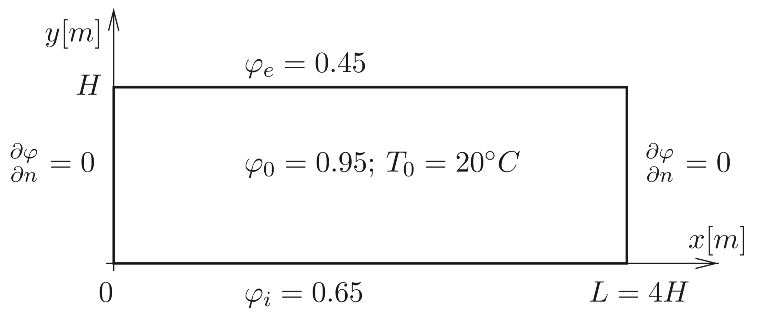
1.2. Boundary conditions
The surounding temperature is constant: \(T_e = T_i = 20^{\circ}C\).
The top (exterior) and bottom (interior) surfaces of the structure are exposed to \(\varphi_e = 45\%\) and \(\varphi_i = 65\%\), respectively.
Homogeneous Neunmann conditions stand on the lesft and right sides of the structure.
1.3. Initial conditions
The initial hygrothermal conditions of the structure are: \(T_0 = 20^{\circ} C\) and \( \varphi = 95 \%\).
1.4. Material properties
-
Sorption isotherm:
-
Vapor diffusion
-
Moisture diffusivity
-
Thermal conductivity
-
Specific hest capacity
-
Density
2. Analytical solution
Under isothermal conditions, the 1D mass transfer equation reads:
its analytical solution is given by:
with
where:
-
\(w_0 = w\left( \varphi_0 \right) = 84.8 ~ kg/m^3\), \(\varphi_0 = \varphi \left( y, t = 0 \right)\)
-
\(w_i = w\left( \varphi_i \right) = 19.5 ~ kg/m^3\), \(\varphi_i = \varphi \left( y = 0, t \right)\)
-
\(w_e = w\left( \varphi_e \right) = 30.5 ~ kg/m^3\), \(\varphi_e = \varphi \left( y = H, t \right)\)
-
\(D_w = 6 \cdot 10^{-10} \quad m^2/s\)
The following figure shows the moisture content profile after 100h, 300h and 1000h obtained with the analytial solution.
The following figure shows the moisture content variation at \(y= \frac{H}{2}\) obtained with the analytial solution.
3. Results from [Škerget2014]
3.1. Time and Space Discretization
Different meshes of \(M=1 \times 4, M=20 \times 10, M=20 \times 20\) and \(M=20 \times 40\) are considered.
The time dependent analysis is performed by running the simulation from the initial state with a time step value of \(\Delta t=1 \mathrm{h}=3600\mathrm{s}\).
The aim is to calculate the moisture distribution after \(t=100,300\) and \(1000 h\).
3.2. Model
At constant moisture diffusivity, mass transfer is controlled according to equation (8) under the following boundary conditions of the first:
and
3.3. Results
Fig. 2 shows the initial moisture content and moisture distribution across the structure at \(t=100,300\) and 1000 h for four different discretization models.
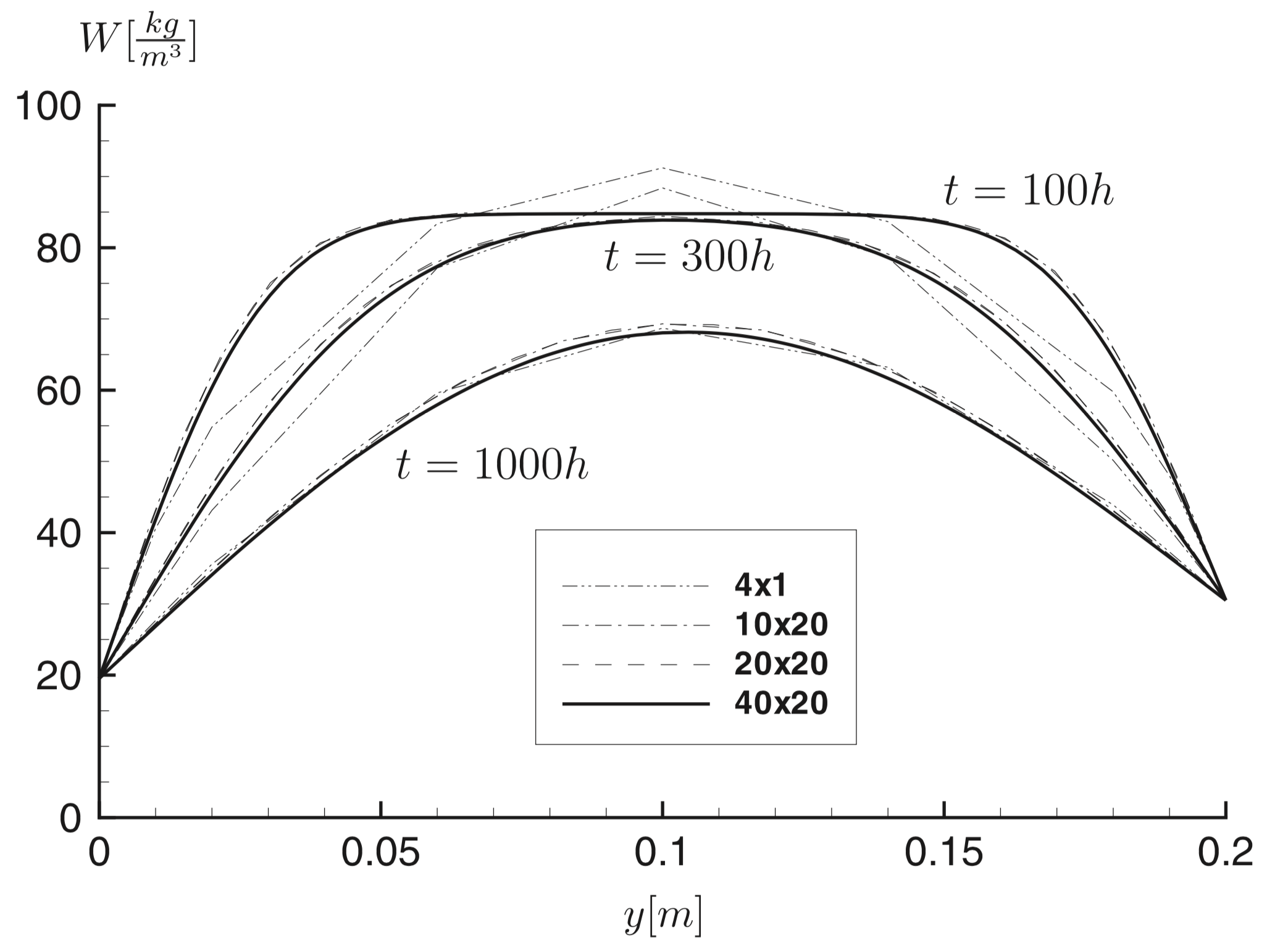
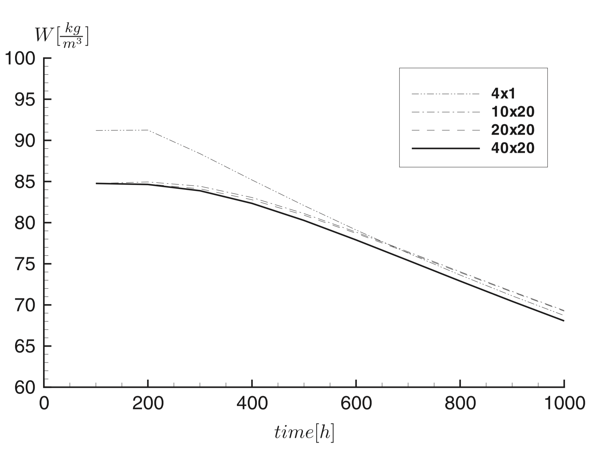
Fig. 3 shows the moisture content variation \(\left(w(t)\right)\) in the middle of the structure \(\left(y=\frac{H}{2}\right)\) for four different discretization models.
3.4. Simulation
To launch the simulation, use this line of code, with those cases files :
mpirun -np 4 ./feelpp_hm_heat_moisture --config-file cases/drying-layer/drying-layer.cfg --mod-file "\$cfgdir/drying-layer.json" --hm.export={360000,1080000,3600000}
3.5. Resolution
The results at \(t=100\)h, \(t=300\)h, \(1000\)h obtained with Feel++ are given on this figure :
The following figure shows the moisture content variation at \(y= \frac{H}{2}\) obtained with the analytial solution.
We can see that for both measures, the results obtained with the application correspond to the analytical solution. It tells us that the model and the code of the application is quite correct !
References
-
[CEN2007] EN 15026, Hygrothermal performance of building components and building elements - Assessment of moisture transfer by numerical simulation, CEN, 2007.
-
[HAM2002] C.-E. Hagentoft, HAMSTAD – Final report: methodology of HAM-modeling, Report R-02:8, Gothenburg, Department of Building Physics, Chalmers University of Technology, 2002.
-
[Kumaran1994] Kumaran, M. K., Mitalas, G. P. and Bomberg, M. T. (1994), 'Fundamentals of transport andstorage of moisture in building materials and components', Trechsel, H. R. (ed), Moisture control in buildings.
-
[KUN1995] Künzel H, Simultaneous Heat and Moisture Transport in Building Components, PhD thesis, Fraunhofer Institute of Building Physics, 1995.
-
[Kunzel2004] Kunzel, H.M., Holm, A., Zirkelbach, D. and Karagiozis, A.N., Simulation of indoor temperature and humidity conditions including hygrothermal interactions with building envelope Solar Energy 78 (2005) 554–561.
-
[Mendes2019] Mendes, N., Chhay, M., Berger, J. and Dutykh, D., Numerical methods for diffusion phenomena in building physics, Springer Nature Switzerland AG 2019.
-
[Neymark2002] Neymark, J. and Judkoff, R. International energy agency building simulation test and diagnostic method for heating, ventilation, and air-conditioning equioement models (HVAC BESTEST). Volume 1: Cases E100-E200 Technical Report NREL/TP-550-30152.
-
[Škerget2014] Škerget, L. and Tadeu, A. BEM numerical simulation of coupled heat and moisture flow through a porous solid Engineering Analysis with Boundary Elements, 2014.
-
[Straube2002] Straube J. F., Moisture in Buildings, ASHRAE Jornal, January 2002.