BESTEST

This benchmark test is taken from [Medens2019].

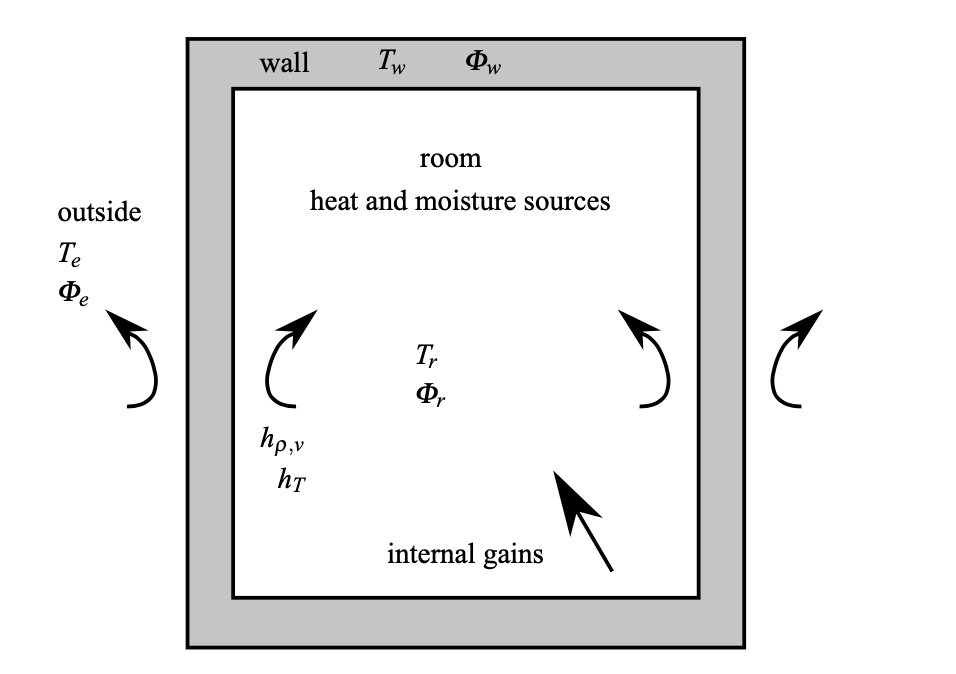
The following involve the coupling between the diffusion transfer in the porous walls and the heat and moisture balances in the room air as illustrated in the fig 1 (right).

1. Building description

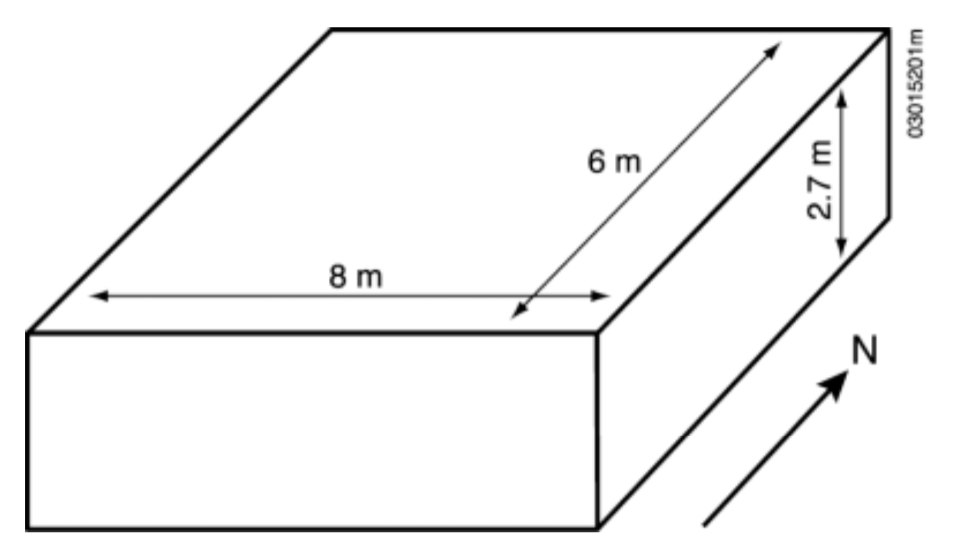
This case study was inspired by the benchmark BESTEST [Neymark2004] where the building geometry (fig. 1 (left)) is descibed. The area of the walls is $75.6 ~\mathrm{m}^{2},$ and that of the roof and floor is $48 ~\mathrm{m}^{2}$ each. Their thicknesses are $0.15 ~\mathrm{m}$.

BESTEST building geometry.

bestgeometry

Radiative transfer is not considered, and the inside and outside surface coefficients are:

\[\begin{array}{ll} h_i=8.29 & \left(\mathrm{W} / \mathrm{m}^{2} . \mathrm{K}\right) \\ h_e=29.30 & \left(\mathrm{W} / \mathrm{m}^{2} . \mathrm{K}\right) \end{array}\]

It is assumed that the floor, roof, and walls are composed of aerated concrete, the properties of which are given in the table below.

Table 1. Dry-basis properties of wall materials
Soil	$\rho_{0}\left(\mathrm{kg} / \mathrm{m}^3\right)$	$c_{m}(\mathrm{J} / \mathrm{kg} . \mathrm{K})$	$\lambda_{m}(\mathrm{W} / \mathrm{m} . \mathrm{K})$
Aerated concrete	650	840	0.18
EPS	10	1450	0.05
Concrete	2500	1000	1

A $100 \%$ convective heat gain of $500\,\mathrm{W}$ between 9 am and 5 pm and a 24 h ventilation rate of $\eta=0.5$ ach are considered.

The initial temperature is set to $20^{\circ} \text{C}$

The exercice is devided into three parts:

First perform a heat transfer simulation alone,
second: perform a moisture transfer simulation alone,
perform a coupled heat and moisture transfer simualation.

2. Heat Transfer

The results should be presented for the 30 th day of simulation to prevent effects imposed by the assumed initial values of temperature $\left(20^{\circ} \mathrm{C}\right)$ and a sinus function to represent the daily variation of external temperature:

\[T_{e}=298.15+\sin (2 \pi t / 86400)\]

Define the governing differential equations of the wall heat diffusion problem and of the inside of room as balanced. Compute the temperature inside the room.
Add an Expanded polystyrene (EPS) insulation material of $5\,\mathrm{cm}$ (properties are given in Table 1 ) on the external side of the building envelope, and compare the temperature profile with and without the material.
Repeat exercise (2) by placing the EPS layer at the internal boundary.
Elaborate a table to summarize the results in terms of daily energy transferred, internal temperature peaks, and delay and damping effects. Compare your results presented with those obtained by running a buildingsimulation software.

2.1. Governing differential equations

We denote by $T_w$ [K] the wall temperature and $T_r$ [K] the room temperature.

2.1.1. Wall heat diffusion

\[\rho_m \cdot c_m \frac{\partial T_w}{\partial t}-\nabla(k\nabla T_w)=0\]

With :

$\rho_m$ [$\mathrm{kg} / \mathrm{m}^3$] is the material density.
$c_m$ [$\mathrm{J} / \left(\mathrm{kg} . \mathrm{K} \right)$] is the material thermal mass capacity.
$k$ [$\mathrm{W} \cdot \mathrm{m}^{-1} \cdot \mathrm{K}^{-1}$] is the thermal conductivity.

Boundary conditions:

All the building walls are subjected to a convective heat transfer on both their inside ($W_i$) and outside ($W_e$) surfaces:

\[\begin{align} \text{On }W_i : & -k\nabla T_w=h_i(T_r-T_{w_{s,i}})\\ \text{On }W_e : & -k\nabla T_w=h_e(T_e-T_{w_{s,e}})\\ \end{align}\]

Where:

$W_i$ is the boundary between the wall and the room, and $W_e$ is the border between the wall and the outside.
$T_{w_{s,i}}$ (resp. $T_{w_{s,e}}$) is the temperature of the wall at its interior (resp. exterior) border.
$h_i$ (resp. $h_e$) is inside (resp. outisde) convective heat transfer coefficient.

2.1.2. Room heat balance

\[\rho_a c_a \frac{\partial T_r}{\partial t} - h_i \cdot A_w \cdot \left( T_{w_{s,i}} - T_r \right) - \eta \cdot \rho_a c_a \cdot V_a \cdot \left( T_e - T_r \right) = H\]

where:

$\rho_a$ [$\mathrm{kg} / \mathrm{m}^3$] is the air density.
$c_a$ [$\mathrm{J} / \left(\mathrm{kg} \cdot \mathrm{K} \right)$] is the air heat capacity.
$V_a$ [$\mathrm{m}^3$] is the room volume.
$\eta$ [$\mathrm{h}^{-1}$] is the ventilation rate.
$h_i$ [$\mathrm{W}/ \left(m^2 \cdot K\right)$] is the inside convective heat transfer coefficient.
$A_w$ [$\mathrm{m}^2$] is the total area of the walls.
$H$ [$\text{W}$] is the heating power.
The term: $ h_i \cdot A_w \cdot \left( T_{w_{s,i}} - T_r \right) $ corresponds to the convective heat exchange with the building walls and the term: $ \eta \cdot \rho_a c_a \cdot V_a \cdot \left( T_e - T_r \right) $ represents the heat flow throught the ventilation.

2.1.3. Final system

The final system, including the walls heat diffusion and the room heat balance reads:

\[\begin{align} \rho_m c_m \frac{\partial T_w}{\partial t}-\nabla\left(k\nabla T_w\right)&=0 \tag{$E_w$}\label{ew}\\ \rho_a c_a\frac{\partial T_r}{\partial t}- h_i (T_{w_{s,i}}-T_r)A_w -\eta\rho_a c_a V_a (T_e-T_r) &= H \tag{$E_r$}\label{er} \end{align}\]

with

$H=\begin{cases}500\,\mathrm{W} \quad \text{if}\, t\, (\text{mod}\, 1\, \text{day}) \in[9\text{h},17\text{h}]\\0\,\mathrm{W}\quad \quad \text{otherwise}\end{cases}$.
$\eta = 0.5$
Boundary conditions on the walls:

\[\left\{ \begin{array}{l} - k\nabla T_w=h_i(T_r-T_{w_{s,i}}) \quad \text{On} ~ W_i\\ - k\nabla T_w=h_e(T_e-T_{w_{s,e}}) \quad \text{On} ~ W_e \end{array} \right.\]

Initial condition: $T_{w_0} = T_{r_0} = 20 ^{\circ} \text{C} $

2.2. Euler scheme

To solve the heat equation for the room, we use a first oder explicit euler scheme :

\[\dfrac{\partial T_r}{\partial t} \approx \dfrac{T_r^{n+1} - T_r^n}{\Delta t}\]

where $\Delta t$ is the time-step, and $T_r^n = T_r(t=n\Delta t)$

The equation $\ref{er}$ becomes :

\[\rho_a c_a\frac{T^{n+1}-T^n}{\Delta t}- h_{i}A_w(T_{w_{s,i}}-T_r^{n+1})A_w - \eta\rho_a c_a V_a(T_e-T_r^{n+1}) = H\]

Which is equivalent to :

\[\left(\frac{\rho_a c_a}{\Delta t}+ h_{i}A_w+\eta\rho_a c_a V_a\right)T_r^{n+1} = H + h_{i}A_wT_{w_{s,i}}+\eta\rho_a c_a V_a T_e + \frac{\rho_a c_a}{\Delta t}T_r^n \tag{$E_{r,Euler}$}\label{er:euler}\]

Technical details for the implementation are available here.

3. Moisture Transfer

We consider the same building model as described in the previous exercise but isothermally at $20^{\circ} \mathrm{C}$. A $500 \mathrm{g} / \mathrm{h}$ indoor moisture production between $9 \mathrm{am}$ and $5 \mathrm{pm},$ and a $24 \mathrm{h}$ ventilation rate of $0.5$ ach is considered.

The moisture properties of the aerated concrete, vapor permeability, and sorption isotherm are as follows:

\[\begin{array}{l} \delta_{v}=3 \cdot 10^{-11} \\ \theta=0.042965 \phi \end{array}\]

The mass convective coefficient based on vapor pressure difference is $h_{m}=$ $0.00275 ~ \mathrm{m} / \mathrm{s}$ for the inside and outside parts of the wall.

The outside conditions for relative humidity are constant and at $30 \% .$

The results should be presented for the 365th day of simulation to prevent effects imposed by the assumed initial values of moisture content as moisture diffuses slowly.

Define the governing differential equations of the wall and the inside of room. In addition, compute the relative humidity inside the room.
Compare the daily relative humidity profile with and without adsorption.
Compare your results with the results from whole-building simulation programs that consider moisture.
What could be the minimum warm-up period to avoid the effects of the initial conditions?

3.1. Governing differential equations

3.1.1. Wall

\[\xi \frac{\partial \phi}{\partial t}+\nabla \cdot\left(-\xi D_{\mathrm{w}} \nabla \phi-\delta_{\mathrm{p}} \nabla\left(\phi p_{\mathrm{sat}}\right)\right)=0\]

where :

$\phi$ [-] is the relative humidity.
$\xi$ [$\mathrm{kg} / \mathrm{m}^{3}$] is the moisture storage capacity.
$\delta_{\mathrm{p}}$ [s] is the vapor permeability.
$p_{\text {sat }}$ [$\mathrm{Pa}$] is the vapor saturation pressure.
$D_{\mathrm{w}}$ [$\mathrm{m}^{2} / \mathrm{s}$] is the moisture diffusivity.

For aerated concrete, we have this relation [Kumaran1996] :

\[D_w = 9.2 \times 10^{-11} \cdot \exp\left(0.0215 w \right)\]

Boudary conditions

Convective mass transfer applies on both the inside and outside surfaces of the walls :

\[\left\{ \begin{array}{l} -\xi D_{\mathrm{w}} \nabla \phi-\delta_{\mathrm{p}} \nabla\left(\phi p_{\mathrm{sat}}\right)= h_{m_i} \left( w_r - w_{s,i} \right) \quad \text{On} ~ W_i\\ -\xi D_{\mathrm{w}} \nabla \phi-\delta_{\mathrm{p}} \nabla\left(\phi p_{\mathrm{sat}}\right)= h_{m_e} \left( w_e - w_{s,e}\right) \quad \text{On} ~ W_e \end{array} \right.\]

where:

$w_r$ and $w_e$ are the room and the outside air relative humidities respectively.
$w_{s_i}$ and $w_{s_e}$ are the relative humidities at the inner and outter surfaces of the walls respectively.
$h_{m_i}$ and $h_{m_e}$ [$\text{m}/\text{s}$] are the the repectively inside and outside mass convective coefficients based on vapor pressure difference. Herein $h_{m_i} = h_{m_e} = h_m$

3.1.2. Room

\[V_a \frac{dw_r}{dt} = \eta \cdot V_a (w_{e} - w_r) + \dot{m}_{gen} + h_m \cdot A_w (w_{s,i} - w_r)\]

where

$V_a$ [$\mathrm{m^3}$] is the room volume.
$h_m$ [$\mathrm{m} / \mathrm{s} $] is the mass convective coefficient based on vapor pressure difference.
$A_{w}$ [$\mathrm{s^2} $] is the total area of the walls.
$\eta$ [$\mathrm{s}^{-1}$] is the ventilation rate.
$\dot{m}_{gen}$ [$\mathrm{kg} / \mathrm{s}$] is the internal water-vapor generation.
$w_{s,i}$ [$\mathrm{kg} / \mathrm{m^3}$ ] is the water content at the internal surface of the walls.
$w_{e}$ [$\mathrm{kg} / \mathrm{m^3}$ ] is the water content of the outside air.
$w_r$ [$\mathrm{kg} / \mathrm{m^3} $] is the water content (absolute humidity )of the room volume.

The water content (or absolute humidity), $w$ [$\text{kg}/\text{m}^3$], is defined as the mass of water vapor, $m_v$ [$\text{kg}$], present per unit of air volume, $V$ [$\text{m}^3$]:

\[w = \frac{m_v}{V}\]

Using the general law for perfect gases leads to the followin:

\[w = \frac{p_v}{R_v \cdot T}\]

where

$p_v$ [$\text{Pa}$] is the partial pressure of water vapor.
$R_v$ [$\text{J} \cdot \text{Kg} \cdot \text{K}$] is the gas constant for water vapor.
$T$ [$\text{K}$] is the ambiant temperature.

3.1.3. Coputing the air relative humidity

The relative humidity is defined as the ratio of partial pressure of the water vapor present at a given temperature and parometric pressure, $p_v$, to the partial pressure of the water present at saturation at a given temperature and pressure, $p_{sat}$:

\[\phi = \frac{p_v}{p_{\text{sat}}}\]

where

$p_v$ [$\text{Pa}$] is the partial pressure of water vapor.
$p_{\text{sat}}$ [$\text{Pa}$] is the partial pressure of water vapor at saturation.

The partial pressure can be deduced from the absolute humidity and used to compute the relative humidity as follows:

\[\phi = \frac{w \cdot R_v \cdot T}{p_{\text{sat}}}\]

4. Heat and Moisture Transfer

Now, both the previous exercises can be considered for coupled heat and moisture transport phenomena, including the latent heat effect.

Solve the combined problem

Write the governing equations for both moisture content and vapor pressure driving potentials.
Quantify the importance of considering moisture by comparing the result with the results of the previous exercises.
How can you consider the effect of rain?
Show quantitatively the effects of a latex paint (see values in Chap.2) on the results of Exercise 3
In your opinion, what are the main challenges in building physics regarding the use of traditional numerical methods applied to diffusion phenomena?

4.1. Governing equation

4.1.1. Wall

We have the following equations for heat and moisture transport throught the wall:

\[\begin{array}{l} \left(\rho_m c_m \right)_{\mathrm{eff}} \frac{\partial T_w}{\partial t}+\nabla \cdot\left(-k_{\mathrm{eff}} \nabla T_w - L_{\mathrm{v}} \delta_{\mathrm{p}} \nabla\left(\phi_w p_{\mathrm{sat}}\right)\right)= 0 \\ \quad \xi \frac{\partial \phi_w}{\partial t}+\nabla \cdot\left(-\xi D_{\mathrm{w}} \nabla \phi_w-\delta_{\mathrm{p}} \nabla\left(\phi_w p_{\mathrm{sat}}\right)\right)= 0 \end{array}\]

Boundary conditions

The floowing boundary conditions apply for the heat transfer:

\[\left\{ \begin{array}{l} - k\nabla T_w=h_i(T_r-T_{w_{s,i}}) + h_m \cdot L_v \left( w_r - w_{s,i} \right) \quad \text{On} ~ W_i\\ - k\nabla T_w=h_e(T_e-T_{w_{s,e}}) + h_m \cdot L_v \left( w_e - w_{s,e} \right) \quad \text{On} ~ W_e \end{array} \right.\]

The boundary conditions for the moisture transfer are as follows:

4.1.2. Room

The following describe the heat and moisture balance of the room air:

\[\begin{array}{l} \rho_a c_a \frac{\partial T_r}{\partial t} - h_i \cdot A_w \cdot \left( T_{w_{s,i}} - T_r \right) - \eta \cdot \rho_a c_a \cdot V_a \cdot \left( T_e - T_r \right) = H\\ V_a \frac{dw}{dt} = \eta \cdot V_a (w_{ext} - w) + \dot{m}_{gen} + h_m \cdot A_w (w_{s,i} - w) \end{array}\]

References

[CEN2007] EN 15026, Hygrothermal performance of building components and building elements - Assessment of moisture transfer by numerical simulation, CEN, 2007.
[HAM2002] C.-E. Hagentoft, HAMSTAD – Final report: methodology of HAM-modeling, Report R-02:8, Gothenburg, Department of Building Physics, Chalmers University of Technology, 2002.
[Kumaran1994] Kumaran, M. K., Mitalas, G. P. and Bomberg, M. T. (1994), 'Fundamentals of transport andstorage of moisture in building materials and components', Trechsel, H. R. (ed), Moisture control in buildings.
[KUN1995] Künzel H, Simultaneous Heat and Moisture Transport in Building Components, PhD thesis, Fraunhofer Institute of Building Physics, 1995.
[Kunzel2004] Kunzel, H.M., Holm, A., Zirkelbach, D. and Karagiozis, A.N., Simulation of indoor temperature and humidity conditions including hygrothermal interactions with building envelope Solar Energy 78 (2005) 554–561.
[Mendes2019] Mendes, N., Chhay, M., Berger, J. and Dutykh, D., Numerical methods for diffusion phenomena in building physics, Springer Nature Switzerland AG 2019.
[Neymark2002] Neymark, J. and Judkoff, R. International energy agency building simulation test and diagnostic method for heating, ventilation, and air-conditioning equioement models (HVAC BESTEST). Volume 1: Cases E100-E200 Technical Report NREL/TP-550-30152.
[Škerget2014] Škerget, L. and Tadeu, A. BEM numerical simulation of coupled heat and moisture flow through a porous solid Engineering Analysis with Boundary Elements, 2014.
[Straube2002] Straube J. F., Moisture in Buildings, ASHRAE Jornal, January 2002.

Soil	\(\rho_{0}\left(\mathrm{kg} / \mathrm{m}^3\right)\)	\(c_{m}(\mathrm{J} / \mathrm{kg} . \mathrm{K})\)	\(\lambda_{m}(\mathrm{W} / \mathrm{m} . \mathrm{K})\)
Aerated concrete	650	840	0.18
EPS	10	1450	0.05
Concrete	2500	1000	1