Data processing and missing data
As part of this internship, we’re collecting lots of data using sensors with the intention to automate decision-making through the strategic use of machine learning. But there are many steps to master in order to build a production AI system.
This data-management (or data processing) work can be broken down into a handful of phases, including:
-
Data discovery: What data we need, and how to find it?
-
Data analysis: Is the data useful for Machine Learning (ML)? How we validate it?
-
Data preparation: What format is the data in? How to transform it into the correct format?
-
Data modeling: What algorithm can we use to model the data?
-
Model evaluation: Is the model working as expected? What changes we need to make?
Unfortunately, in Data Science projects, data often contain outliers and missing data.
It is important to identify the missing data in a dataset before applying a Machine Learning (ML) algorithm. This is because many ML algorithms rely on statistical methods that assume a complete dataset as input. Otherwise, the ML algorithm may provide a poor predictive model or worse, simply not work. Thus, dealing with missing data is a necessary phase for any Data Science project.
1. Missing data
Machine Learning’s algorithms take the input data in matrix form, each row is an observation, and each column represents a feature of the individual.
An observation (row of the data matrix) is said to have missing data if there is a feature for which its value is not filled in.
Missing data is a problem that manifests itself not only in Data Science but also in statistical modelling. The aim is to find out how to process these missing data in such a way as to complete the missing information without significantly altering the original data set.
This is why we use missing data imputation, which refers to replacing missing values in the dataset with artificial values. Ideally, these replacements should not lead to a significant alteration in the distribution and composition of the dataset.
This is where machine learning algorithms such as Random Forest (RF used in the second semester project), or Recurrent Neural Networks (RNN) are used, using the different tools presented in this link.
Within the framework of this internship, the study was carried out on one of the API Cluster located in the Innovation Park of Illkirch-Graffenstaden, by collecting physical data (temperature, light, humidity, sound and pir) from 71 sensors placed at the level of the building. The data imputation was carried out by applying a type of recurrent neural networks called Long Short Term Memory (LSTM). [Missing_data]
2. Long Short Term Memory (LSTM)
2.1. Introduction
Recurrent Neural Networks suffer from short-term memory. If a sequence is long enough, they’ll have a hard time carrying information from earlier time steps to later ones.
During back propagation, recurrent neural networks suffer from the vanishing gradient problem. Gradients are values used to update a neural networks weights. The vanishing gradient problem is when the gradient shrinks as it back propagates through time. If a gradient value becomes extremely small, it doesn’t contribute too much learning.
So in recurrent neural networks, layers that get a small gradient update stops learning. Those are usually the earlier layers. So because these layers don’t learn, RNN’s can forget what it seen in longer sequences, thus having a short-term memory.
LSTM ’s were created as the solution to short-term memory. They have internal mechanisms called gates that can regulate the flow of information. These gates can learn which data in a sequence is important to keep or throw away. By doing that, it can pass relevant information down the long chain of sequences to make predictions.
2.2. Operating process of an lstm cell
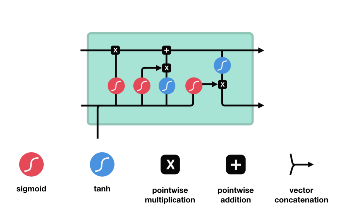
We have three different gates that regulate information flow in an LSTM cell. A forget gate, input gate, and output gate.[LSTM]
-
Forget gate : This gate decides what information should be thrown away or kept. Information from the previous hidden state and information from the current input is passed through the sigmoid function. Values come out between 0 and 1. The closer to 0 means to forget, and the closer to 1 means to keep.
-
Input gate : First, we pass the previous hidden state and current input into a sigmoid function. That decides which values will be updated by transforming the values to be between 0 and 1. 0 means not important, and 1 means important. We also pass the hidden state and current input into the tanh function to squish values between -1 and 1 to help regulate the network. Then we multiply the tanh output with the sigmoid output. The sigmoid output will decide which information is important to keep from the tanh output.
-
Cell state : First, the cell state gets pointwise multiplied by the forget vector. This has a possibility of dropping values in the cell state if it gets multiplied by values near 0. Then we take the output from the input gate and do a pointwise addition which updates the cell state to new values that the neural network finds relevant. That gives us our new cell state.
-
Output gate : It decides what the next hidden state should be. First, we pass the previous hidden state and the current input into a sigmoid function. Then we pass the newly modified cell state to the tanh function. We multiply the tanh output with the sigmoid output to decide what information the hidden state should carry. The output is the hidden state. The new cell state and the new hidden is then carried over to the next time step.
To get more informations about the mechanics of LSTM, you can follow the link.
3. Application
In the framework of our training course, we used the different methods of machine learning, going through the different steps of data processing, and using the necessary tools in order to create a colab notebook that makes univariate and multivariate time series predictions.
3.1. Data extraction
The first step is to import the necessary librairies that will allow us to carry out our study.
Then we import the data from the lstm_data csv file contained in the synapse-data github repository.
This csv file contains the different physical fields (temperature, humidity, light, pir and sound) for all the nodes collected every hour for a period of one year (starting from 01/01/2019) by exploiting the following link.