Application feelpp_hm_heat_moisture devlopment
As is it coded yet, the application feelpp_hm_heat_moisture can only be used for one of the previous benchmarks at a time (drying-layer, and moisture-uptake) : the values of the parameters are distinguished with macros, and we have to build again if we want to chang e, which is not a good strategy !
The idea is now to adapt it to make it work for all types of problems we want to model, using a JSON file.
1. Complete variationnal problem
We considere the problem of heat-moisture transport (cf here) :
This system of equations is satisfied on the domain \(\Omega\). We add those boundary counditions :
We have \(\partial\Omega=\Gamma_{T,D}\cup\Gamma_{T,N}\), and \(\partial\Omega=\Gamma_{\phi,D}\cup\Gamma_{\phi,N}\).
We make the usual time derivate approximation : \(\dfrac{\partial T}{\partial t}\approx\dfrac{T^{n+1}-T^n}{\Delta t}\)
Let \(v\) be a test function associated to \(T\). The first equation \(\ref{eq:T}\) become, after making a partial integration :
As \(v=0\) on \(\Gamma_{T,D}\) and on \(\Gamma_{\phi,D}\), and also there are the two Neimann conditions, this equation become :
with :
-
\(a(T^{n+1},v) = \displaystyle\int_\Omega (\rho C_p)_\mathrm{eff}^n\dfrac{T^{n+1}}{\Delta t}v + \int_\Omega(k_\mathrm{eff}^n\nabla T^{n+1})\nabla v\)
-
\(b(\phi^{n+1},v) = \displaystyle\int_\Omega L_v^n\delta_\mathrm{p}^np_\mathrm{sat}^n\nabla\phi^{n+1}\nabla v + \int_\Omega L_v^n\delta_\mathrm{p}^n\nabla p_\mathrm{sat}^n \phi^{n+1}\nabla v - \int_{\Gamma_{\phi,N}}\left(L_v^n\delta_\mathrm{p}^n\nabla p_\mathrm{sat}^n\phi^{n+1}\cdot\mathbf{n}\right)v\)
-
\(f(v) = \displaystyle\int_\Omega \left((\rho C_p)_\mathrm{eff}^n\dfrac{T^n}{\Delta t} + Q^{n+1}\right)v + \int_{\Gamma_{T,N}} k_\mathrm{eff}^n N_T^{n+1} v + \int_{\Gamma_{\phi,N}} L_v^n\delta_\mathrm{p}^n\nabla p_\mathrm{sat}^n N_\phi^{n+1} v\)
Doing the same process with a test function \(q\) associated to \(\phi\), the equation \(\ref{eq:phi}\) become :
with :
-
\(d(\phi^{n+1},q) = \displaystyle\int_\Omega\xi^n\frac{\phi^{n+1}}{\Delta t}q + \int_\Omega\xi^nD_\mathrm{w}^n\nabla\phi^{n+1}\nabla q + \int_\Omega\delta_\mathrm{p}^n\nabla\phi^{n+1}p_\mathrm{sat}^n\nabla q + \int_\Omega\delta_\mathrm{p}^n\phi^{n+1}\nabla p_\mathrm{sat}^{n}\nabla q - \int_{\Gamma_{N,\phi}}\left(\delta_\mathrm{p}^n\phi^{n+1}\nabla p_\mathrm{sat}^n\cdot\mathbf{n}\right)q\)
-
\(g(q) = \displaystyle\int_\Omega\left(\xi^n\dfrac{\phi^n}{\Delta t} + G^{n+1}\right)q + \int_{\Gamma_{N,\phi}}\left(\xi^nD_\mathrm{w}^n+\delta_\mathrm{p}^np_\mathrm{sat}^n\right)N_\phi^{n+1}q\)
2. Model properties
As explained in the Feel Tutorial Dev, the same set of equation allow solving a lot of different problems. That is why we define a model in Feel.
Models are represented by a class ModelProperties which contains sub-classes corresponding to the different sections of a JSON file. For example, I will show how to do it with boundary conditions, but the process is quite similar.
This object is stored as a member of the class HeatMoisture, named props_.
3. Example of usage for boundary conditions
"BoundaryConditions":
{
    "field":                    (1)
    {
        "BC_type":              (2)
        {
            "marker":           (3)
            {
                "expr":"value"  (4)
            }
        }
}| 1 | field is the field on what the boundary condition is applied (phi for relative humidity or T for heat) |
| 2 | BC_type is the type of boundary condition applied to the field (Dirichlet or Neumann) |
| 3 | marker is the name of the physical entity in the geo file, on which the condition is applied |
| 4 | value is the expression of the value of the condition applied to the field. For Dirichlet condition, it is equal to the value above it, and for Neumann condition, it is the value of \(f\) such as \(\frac{\partial \phi}{\partial n}=f\). |
The boundary conditions are used in the code at the definition of the forms, in the functions update of the two classes (see section 5.3 of the project report)
We distinguich three type of physics used in the model :
-
heat, meaning that we solve only the heat problem -
moisture, meaning that we solve only the moisture problem -
heat-moisture, combining the two problems
We define the physics in the JSON file in a section Materials, on associated markers, allowing to combine physics in a more complex geometry :
"Materials":
{
    "Omega":
    {
        "physics":["moisture"],
        "markers":["Omega"],
    }
}
Let’s focus on the implementation in C++ of the boundary conditions. Here is the (compacted) code of the update function in the class Heat.
void update( double t, PhiT const& phi, double dt )
{
    this->a_.zero() ;
    this->l_.zero() ;

    for ( auto const& [name, mat] : this->props_.materials() ) (1)
    {
        if ( mat.hasPhysics( "heat" ) || mat.hasPhysics( "heat-moisture" ) ) (2)
        {
            // don't depend on boundary conditions
            this->a_ += integrate( _range = markedelements( this->mesh(), mat.meshMarkers() ),
                                   _expr = ... );
            this->l_ += integrate( _range = markedelements( this->mesh(), mat.meshMarkers() ),
                                   _expr = ... );

            if ( mat.hasPhysics( "moisture" ) || mat.hasPhysics( "heat-moisture" ) ) (2)
            {
                this->l_ += integrate( _range = markedelements( this->mesh(), mat.meshMarkers() ),
                                       _expr = ... );
            }

            // depend on the boundary conditions
            for (auto const& [bcid, bc] : this->props_.boundaryConditions2().flatten()) (3)
            {
                if (bcid.type() == "Neumann")
                {
                    if (bcid.field() == "T")    // for heat
                        this->l_ += integrate( _range = markedfaces( this->mesh(), bc.markers() ), _expr = ... );
                    if ( bcid.field() == "phi" && (mat.hasPhysics( "moisture" ) || mat.hasPhysics( "heat-moisture" )) )  // for moisture
                        this->l_ += integrate( _range = markedfaces( this->mesh(), bc.markers() ), _expr = .... );
                }
            }

            for (auto const& [bcid, bc] : this->props_.boundaryConditions2().flatten()) (4)
            {
                if (bcid.type() == "Dirichlet" && bcid.field() == "T")
                {
                    auto Ts = expr( bc.expression() ) ;
                    Ts.setParameterValues({"t",t}) ;
                    this->a_ += on( _range=markedfaces(this->mesh(), bc.markers()), _rhs=this->l_, _element=T_, _expr=Ts) ;
                }

            }
        }
    }
}| 1 | We begin by making a loop on all the materials. |
| 2 | If this material has the physic heat (or heat-moisture), we apply the conditions (and idem for the moisture term). |
| 3 | We make a loop on all the boundary conditions, adding in a first time the terms of Neumann conditions |
| 4 | Finally, we make a second loop on the boundary conditions, because we have to finish by adding the Dirichlet conditions. |
4. Difficulties encountered
With all those modifications, the application work on the first try on the case drying-layer involving only the moisture transport process, but didn’t worked on moisture-uptake : after a few steps, the linear solver of Feel++ didn’t converge, and therefore the results were totally false !
When we try to compare the values of the coefficients got from this simulation and the one got on the application when it was working (without the json file, it correspond to this this state in the history), we see that atfer the first step there are mistakes. The main hypothesis of such error is because we use here expression depending on other expression : for instance, K depends on w, and w depends on phi. There is a fonctionnality in Feel++ allowing to do refactoring, which is still in development : we have to be in the branch features/refactoring of the repository feelpp.
And, of course, there were parenthesis mistakes that made the solutions false ! Once corrected, all worked quite correctly !
5. Documentation of the application
The documentation of the application feelpp_hm_heat_moisture can be found here.
6. Test on several physics
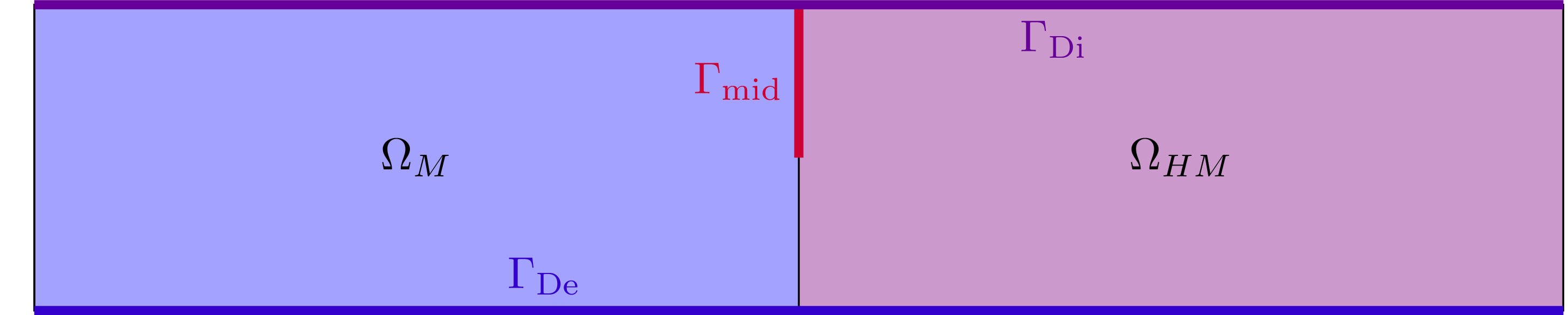
We watch here a created case, with no real correspondance in physic. It is a mix between the two previous cases, moisture-uptake and drying-layer. The geometry is represented on figure 1 : on the left domain \(\Omega_M\), the physic moisture of the drying-layer case is applied, and on the right one \(\Omega_{HM}\), the physic heat-moisture is applied. Moreover, we add a Dirichlet condition on the edge \(\Gamma_\mathrm{mid}\) with \(\phi=0.95\).
In figure 2 is represented the water content after a simulation of 7 days.
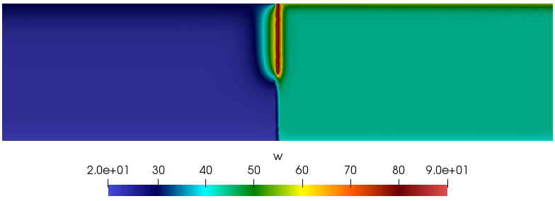
What we see is not relevant in physic, but we figure that the results of the application are coherent.